ホーム » 統計検定1級 2022年 統計数理
「統計検定1級 2022年 統計数理」カテゴリーアーカイブ
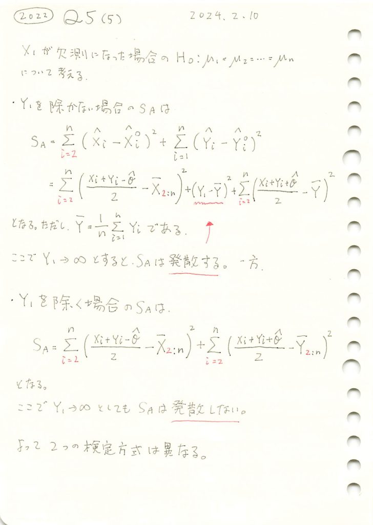
2022 Q5(5)
欠損値がある場合の、分散分析に於けるF検定の影響に関する問をもう一問やりました。
コード
シミュレーションによる計算
# 2022 Q5(5)  2024.8.17

import numpy as np

# シミュレーションの設定
np.random.seed(42)
n = 5  # サンプル数
X = np.random.normal(10, 2, n)  # Xの観測値

# Y1が非常に大きな値を取るケースを考慮
Y = np.random.normal(15, 2, n)
Y[0] = 1000  # Y1が非常に大きな値を取る設定

# 全体平均とY2:nの平均
Y_bar = np.mean(Y)  # 全体の平均
Y_bar_2n = np.mean(Y[1:])  # Y2:n の平均
X_bar_2n = np.mean(X[1:])  # X2:n の平均

# θの推定値
theta_hat = Y_bar_2n - X_bar_2n

# SAの計算(Y1を含める場合)
SA_with_Y1 = np.sum(((X[1:] + Y[1:] - theta_hat) / 2 - X_bar_2n) ** 2) + (Y[0] - Y_bar) ** 2
SA_with_Y1 += np.sum(((X[1:] + Y[1:] + theta_hat) / 2 - Y_bar) ** 2)

# SAの計算(Y1を除く場合)
SA_without_Y1 = np.sum(((X[1:] + Y[1:] - theta_hat) / 2 - X_bar_2n) ** 2)
SA_without_Y1 += np.sum(((X[1:] + Y[1:] + theta_hat) / 2 - Y_bar_2n) ** 2)

# 結果を表示
{
    "Y1を含めた場合の要因A平方和 (SA)": SA_with_Y1,
    "Y1を除いた場合の要因A平方和 (SA)": SA_without_Y1
}
{'Y1を含めた場合の要因A平方和 (SA)': 774276.0933538243,
'Y1を除いた場合の要因A平方和 (SA)': 1.6720954914667048}2022 Q5(4)
欠損値がある場合の、分散分析に於けるF検定の影響に関する問をやりました。

コード
シミュレーションによる計算
# 2022 Q5(4)  2024.8.16

import numpy as np

# シミュレーションのための設定
np.random.seed(42)
n = 5  # サンプル数
X = np.random.normal(10, 2, n)  # Xの観測値
Y = np.random.normal(15, 2, n)  # Yの観測値

# ケース1: Y1を含めた場合の計算
mu_0_1 = Y[0]  # Y1に対応する μ_0
mu_i_with_Y1 = (X[1:] + Y[1:]) / 2  # 残りの μ_i の計算
SE_with_Y1 = np.sum((X[1:] - mu_i_with_Y1) ** 2) + np.sum((Y[1:] - mu_i_with_Y1) ** 2)

# Y1に対する特別な処理
SE_with_Y1 += (Y[0] - mu_0_1) ** 2  # Y1 の影響を追加

# ケース2: Y1を除いた場合の計算
mu_i_without_Y1 = (X[1:] + Y[1:]) / 2  # Y1を除いた場合の μ_i の計算
SE_without_Y1 = np.sum((X[1:] - mu_i_without_Y1) ** 2) + np.sum((Y[1:] - mu_i_without_Y1) ** 2)

# 要因Bに関する平方和(SB)の計算
mu_B_with_Y1 = np.mean(Y[1:])  # Y1を含めた場合のBの平均
mu_B_without_Y1 = np.mean(Y[1:])  # Y1を除いた場合のBの平均

# Y1専用の平均を計算してY1の寄与を計算
mu_0_Y1 = Y[0]  # Y1専用の平均はY1自体
SB_with_Y1 = np.sum((Y[1:] - mu_B_with_Y1) ** 2)
SB_with_Y1 += (Y[0] - mu_0_Y1) ** 2  # Y1の寄与を専用の平均で追加

SB_without_Y1 = np.sum((Y[1:] - mu_B_without_Y1) ** 2)

# 結果を表示
{
    "Y1を含めた場合の残差平方和 (SE)": SE_with_Y1,
    "Y1を除いた場合の残差平方和 (SE)": SE_without_Y1,
    "Y1を含めた場合の要因B平方和 (SB)": SB_with_Y1,
    "Y1を除いた場合の要因B平方和 (SB)": SB_without_Y1,
}
{'Y1を含めた場合の残差平方和 (SE)': 71.28917221001626,
'Y1を除いた場合の残差平方和 (SE)': 71.28917221001626,
'Y1を含めた場合の要因B平方和 (SB)': 8.53547835010338,
'Y1を除いた場合の要因B平方和 (SB)': 8.53547835010338}コメント
Y[0] – mu_0_1 と Y[0] – mu_0_Y1 が0になるので、Y1の有無が結果に影響しない。
2022 Q5(3)
分散分析の各要因の効果を検定する検定量と帰無分布を求めました。
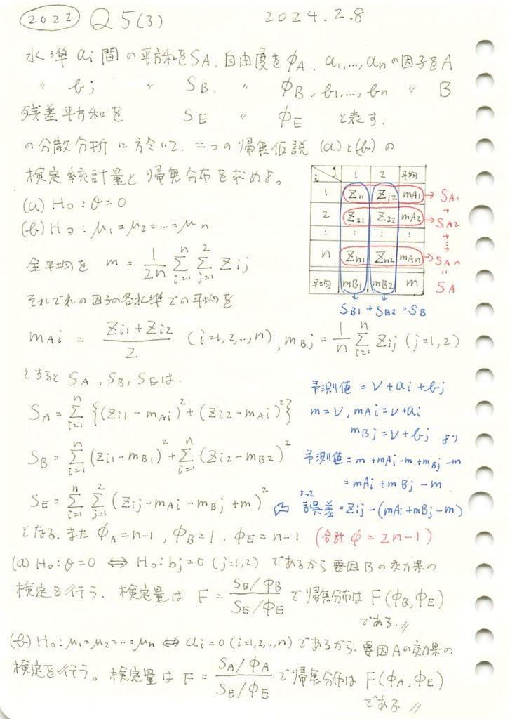
コード
シミュレーションによる計算
# 2022 Q5(3)  2024.8.15

import numpy as np
import pandas as pd
import scipy.stats as stats

# シミュレーションのための設定
np.random.seed(42)
n = 10  # 因子Aの水準数
mu_A = [5, 10, 15]  # 因子Aの水準ごとの平均
mu_B = [7, 12]  # 因子Bの水準ごとの平均
sigma = 2  # 標準偏差
n_samples = n * 2  # 各水準ごとのサンプル数

# データ生成
data = np.zeros((n, 2))
for i in range(n):
    data[i, 0] = np.random.normal(mu_A[i % len(mu_A)], sigma)  # 因子A
    data[i, 1] = np.random.normal(mu_B[i % len(mu_B)], sigma)  # 因子B

# データフレームにまとめる
df = pd.DataFrame(data, columns=['A', 'B'])

# 全平均
m = df.mean().mean()

# 各水準での平均
m_Ai = df['A'].mean()
m_Bj = df['B'].mean()

# 偏差平方和の計算
SA = np.sum((df['A'] - m_Ai) ** 2)
SB = np.sum((df['B'] - m_Bj) ** 2)
SE = np.sum((df.values - m_Ai - m_Bj + m) ** 2)

# 自由度
phi_A = n - 1
phi_B = 1
phi_E = n - 1

# 分散分析の統計量
F_A = (SA / phi_A) / (SE / phi_E)
F_B = (SB / phi_B) / (SE / phi_E)

# p値の計算
p_A = 1 - stats.f.cdf(F_A, phi_A, phi_E)
p_B = 1 - stats.f.cdf(F_B, phi_B, phi_E)

# 結果の表示
{
    "F_A": F_A,
    "p_A": p_A,
    "F_B": F_B,
    "p_B": p_B,
    "SA": SA,
    "SB": SB,
    "SE": SE,
    "df_A": phi_A,
    "df_B": phi_B,
    "df_E": phi_E
}
{'F_A': 0.5528514017044434,
'p_A': 0.8047382043674255,
'F_B': 4.023821861099081,
'p_B': 0.07582222108466219,
'SA': 139.17265361165713,
'SB': 112.54902298706004,
'SE': 251.73609614190576,
'df_A': 9,
'df_B': 1,
'df_E': 9}2022 Q5(2)
分散分析モデルのパラメータを求める問題をやりました。
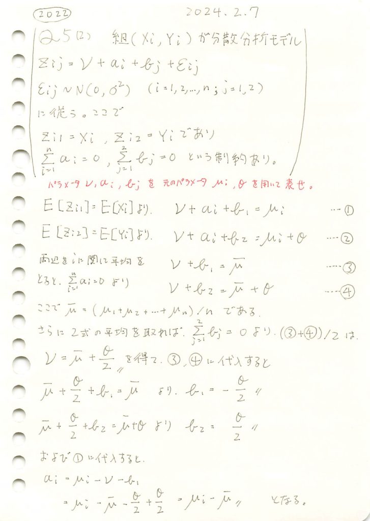
コード
# 2022 Q5(2) 2024.8.14
import sympy as sp
# サンプル数を具体的な数値に設定
n = 3 # 例として n = 3 とする
# シンボリック変数の定義
mu = sp.symbols(f'mu_1:{n+1}') # mu_1, mu_2, mu_3 を定義
theta, nu = sp.symbols('theta nu')
a = sp.symbols(f'a_1:{n+1}') # a_1, a_2, a_3 を定義
b1, b2 = sp.symbols('b1 b2')
# 制約条件
constraint_a = sp.Eq(sum(a), 0)
constraint_b = sp.Eq(b1 + b2, 0)
# Z_{i1} = X_i の関係式
eq1 = sp.Eq(nu + a[0] + b1, mu[0])
# Z_{i2} = Y_i の関係式
eq2 = sp.Eq(nu + a[0] + b2, mu[0] + theta)
# b1, b2 の解を求める
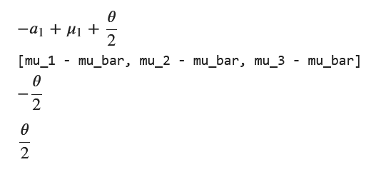
solution_b = sp.solve([constraint_b, b2 - b1 - theta], (b1, b2))
b1_solution = solution_b[b1]
b2_solution = solution_b[b2]
# νとa_iを求めるための方程式
nu_a_eq = eq1.subs({b1: b1_solution})
# νを求める
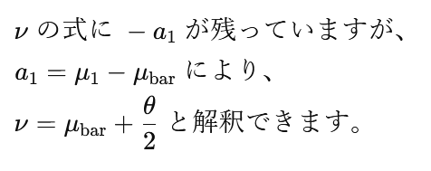
nu_solution = sp.solve(nu_a_eq, nu)[0]
# a_iの解
a_solution = [mu[i] - sp.symbols('mu_bar') for i in range(n)]
# 結果を表示
display(nu_solution, a_solution, b1_solution, b2_solution)
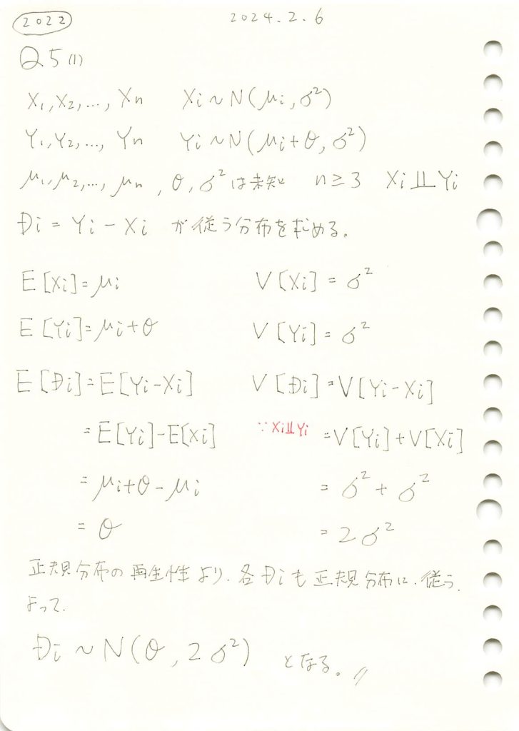
2022 Q5(1)
正規分布の差の分布を求める問題をやりました。
コード
シミュレーションによる計算
# 2022 Q4(5)  2024.8.13

import numpy as np
import matplotlib.pyplot as plt
import scipy.stats as stats

# パラメータの設定
mu_i = 5.0  # 平均値 mu_i
theta = 3.0  # シフトパラメータ θ
sigma = 1.0  # 標準偏差 σ
n = 1000  # サンプル数

# X_i と Y_i のサンプル生成
X_i = np.random.normal(mu_i, sigma, n)
Y_i = np.random.normal(mu_i + theta, sigma, n)

# D_i の計算
D_i = Y_i - X_i

# シミュレーション結果の平均と分散を計算
mean_simulation = np.mean(D_i)
variance_simulation = np.var(D_i)

# 理論上の平均と分散
mean_theoretical = theta
variance_theoretical = 2 * sigma**2

# 結果の表示
print(f"シミュレーション結果: 平均 = {mean_simulation}, 分散 = {variance_simulation}")
print(f"理論値: 平均 = {mean_theoretical}, 分散 = {variance_theoretical}")

# サンプルのヒストグラムを作成
plt.hist(D_i, bins=30, density=True, alpha=0.6, color='g', label='サンプルデータ')

# 理論上の分布を重ねる
x = np.linspace(min(D_i), max(D_i), 1000)
plt.plot(x, stats.norm.pdf(x, mean_theoretical, np.sqrt(variance_theoretical)), 'r', label='理論的な確率密度関数')

plt.title("差 $D_i = Y_i - X_i$ の分布")
plt.xlabel("$D_i$")
plt.ylabel("密度")
plt.legend()
plt.show()
シミュレーション結果: 平均 = 2.975536685240219, 分散 = 2.005575154363111
理論値: 平均 = 3.0, 分散 = 2.0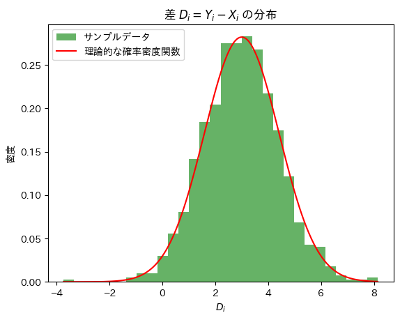
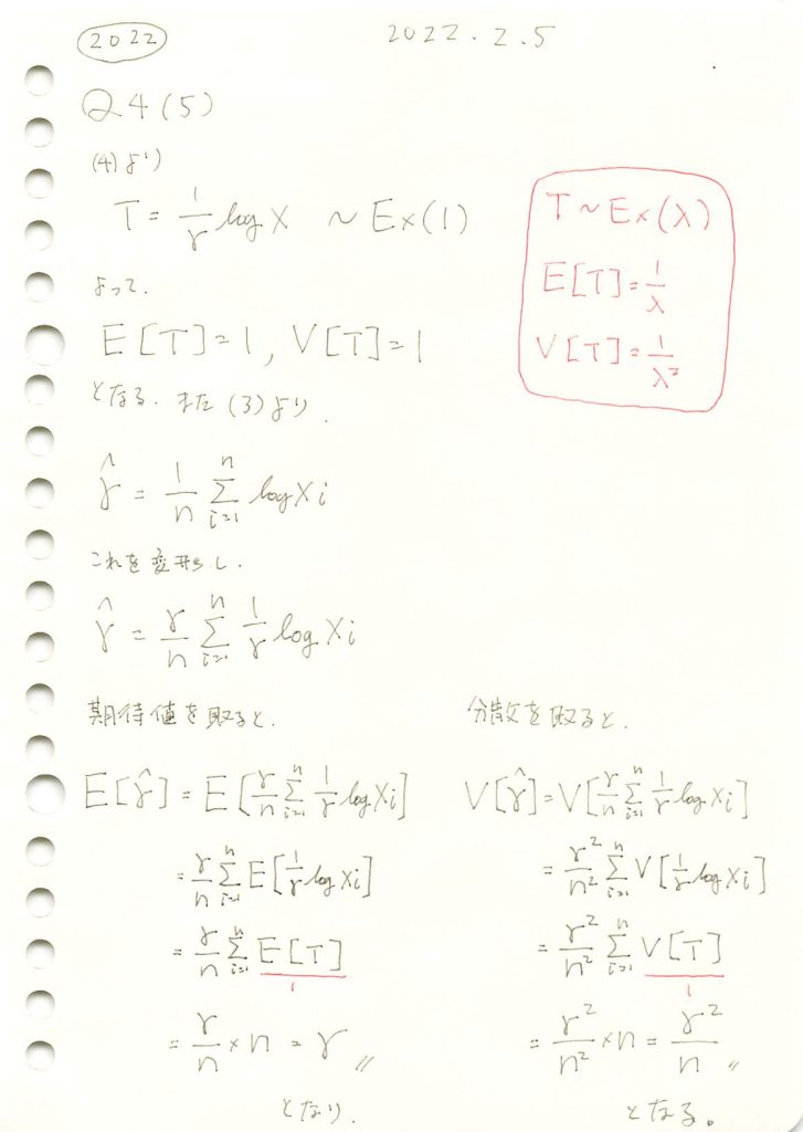
2022 Q4(5)
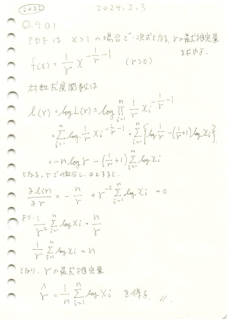
パラメータの推定量の期待値と分散を求めました。
コード
数式を使った計算
# 2022 Q4(5)  2024.8.12

import sympy as sp

# シンボリック変数の定義
gamma = sp.Symbol('gamma', positive=True)
x = sp.Symbol('x', positive=True)

# 確率密度関数 f_X(x) の定義
f_X = (1/gamma) * x**(-(1/gamma + 1))

# E[log X] の計算
E_log_X = sp.integrate(sp.log(x) * f_X, (x, 1, sp.oo))

# E[(log X)^2] の計算
E_log_X2 = sp.integrate((sp.log(x))**2 * f_X, (x, 1, sp.oo))

# V[log X] の計算
V_log_X = E_log_X2 - E_log_X**2

# E[hat_gamma] と V[hat_gamma] の計算
n = sp.Symbol('n', positive=True, integer=True)
E_hat_gamma = E_log_X
V_hat_gamma = V_log_X / n

# 結果の表示
display(E_hat_gamma, V_hat_gamma)

# LaTeXで表示できなときは、こちら
#sp.pprint(E_hat_gamma, use_unicode=True)
#sp.pprint(V_hat_gamma, use_unicode=True)
シミュレーションによる計算
# 2022 Q4(5)  2024.8.12

import numpy as np
import scipy.stats as stats
import matplotlib.pyplot as plt

# パラメータ設定
gamma_true = 1.0  # 真のγの値
n = 100  # サンプルサイズ
num_simulations = 10000  # シミュレーションの回数

# 最尤推定量 \hat{gamma} を格納するリスト
gamma_hats = []

# シミュレーションの実行
for _ in range(num_simulations):
    # 累積分布関数 F(x) に従う乱数を生成
    X = np.random.uniform(size=n)**(-gamma_true)

    # \hat{gamma} の計算
    gamma_hat = np.mean(np.log(X))
    gamma_hats.append(gamma_hat)

# シミュレーション結果の期待値と分散
E_hat_gamma_sim = np.mean(gamma_hats)
V_hat_gamma_sim = np.var(gamma_hats)

# 理論値を計算
# 理論値の計算は、sympyを使って導出した結果を使用
E_hat_gamma_theoretical = 1 / gamma_true  # gammaが1の場合は1が期待値になります
V_hat_gamma_theoretical = (np.pi ** 2) / (6 * n * gamma_true**2)

# 結果の表示
print(f"シミュレーションによる期待値 E[hat_gamma]: {E_hat_gamma_sim}")
print(f"シミュレーションによる分散 V[hat_gamma]: {V_hat_gamma_sim}")
print(f"理論値による期待値 E[hat_gamma]: {E_hat_gamma_theoretical}")
print(f"理論値による分散 V[hat_gamma]: {V_hat_gamma_theoretical}")

# ヒストグラムのプロット
plt.hist(gamma_hats, bins=50, density=True, alpha=0.6, color='g')
plt.axvline(E_hat_gamma_sim, color='r', linestyle='dashed', linewidth=2, label='シミュレーション平均')
plt.axvline(E_hat_gamma_theoretical, color='b', linestyle='dashed', linewidth=2, label='理論値')
plt.xlabel(r'$\hat{\gamma}$の値')
plt.ylabel('密度')
plt.title(r'$\hat{\gamma}$の分布')
plt.legend()
plt.show()
シミュレーションによる期待値 E[hat_gamma]: 0.9995206635186084
シミュレーションによる分散 V[hat_gamma]: 0.010015979040467726
理論値による期待値 E[hat_gamma]: 1.0
理論値による分散 V[hat_gamma]: 0.016449340668482262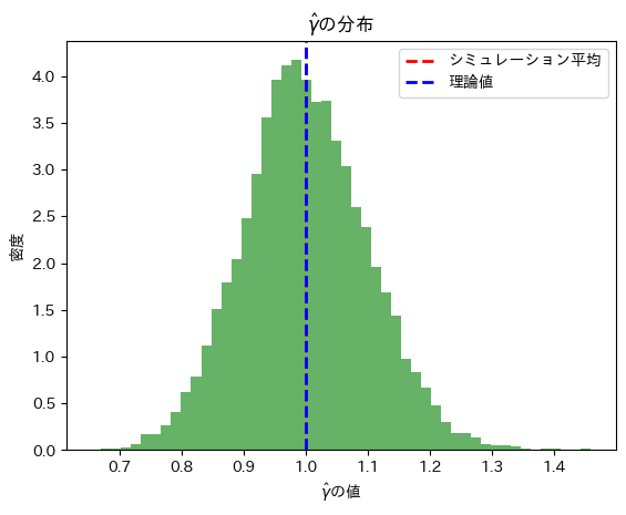
アルゴリズム
サンプル生成:
X = np.random.uniform(size=n)**(-gamma_true)で累積分布関数 F(x) に従う乱数を生成します。逆関数法を使用しています。
最尤推定量の計算:
gamma_hat = np.mean(np.log(X))で各サンプルから計算された をリスト
をリスト gamma_hatsに格納します。
シミュレーション結果の期待値と分散:
- シミュレーション結果の期待値と分散を
E_hat_gamma_simとV_hat_gamma_simに計算し、理論値と比較します。
理論値との比較:
- 理論値を計算して表示し、シミュレーション結果と比較します。
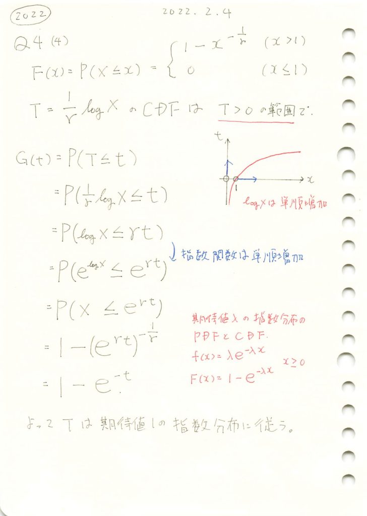
2022 Q4(4)
対数で変数変換した場合の分布を求めました。
コード
数式を使った計算
# 2022 Q4(4)  2024.8.11

import sympy as sp

# シンボリック変数の定義
t, gamma = sp.symbols('t gamma', positive=True)
x = sp.symbols('x', real=True, positive=True)

# 累積分布関数 F_X(x) の定義
F_X = sp.Piecewise((0, x <= 1), (1 - x**(-1/gamma), x > 1))

# F_T(t) の計算
F_T = F_X.subs(x, sp.exp(gamma * t))

# f_T(t) の計算(F_T(t) を t で微分)
f_T = sp.diff(F_T, t)

# 結果の表示
display(F_T, f_T)

# LaTeXで表示できなときは、こちら
#sp.pprint(F_T, use_unicode=True)
#sp.pprint(f_T, use_unicode=True)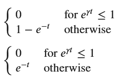
シミュレーションによる計算
# 2022 Q4(4)  2024.8.11

import numpy as np
import matplotlib.pyplot as plt
import scipy.stats as stats

# パラメータ設定
gamma = 1.0  # γの値(例えば1)
num_samples = 10000  # サンプルサイズ

# 累積分布関数 F(x) に従う乱数を生成
X = (np.random.uniform(size=num_samples))**(-gamma)

# T = (1/γ) * log(X) の計算
T = (1/gamma) * np.log(X)

# ヒストグラムをプロット
plt.hist(T, bins=50, density=True, alpha=0.6, color='g', label="シミュレーションによる T")

# 理論的な指数分布の密度関数をプロット
x = np.linspace(0, 8, 100)
pdf = stats.expon.pdf(x)  # 指数分布(λ=1)の密度関数
plt.plot(x, pdf, 'r-', lw=2, label='指数分布の理論値')

# グラフの設定(日本語でキャプションとラベルを設定)
plt.xlabel('Tの値')
plt.ylabel('確率密度')
plt.title(r'$T = \frac{1}{\gamma} \log X$ のヒストグラムと指数分布の比較')
plt.legend()
plt.show()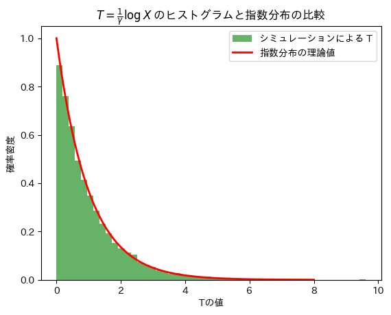
2022 Q4(3)
対数尤度関数を用いてパラメータの最尤推定量を求めました。
コード
数式を使った計算
# 2022 Q4(3)  2024.8.10

import sympy as sp

# シンボリック変数の定義
gamma = sp.Symbol('gamma', positive=True)
n = 10  # 具体的なサンプル数を設定
X = sp.symbols('X1:%d' % (n+1), positive=True)  # X1, X2, ..., Xn を定義

# 尤度関数の定義
L_gamma = sp.prod((1/gamma) * X[i]**(-(1/gamma + 1)) for i in range(n))

# 対数尤度関数の定義
log_L_gamma = sp.log(L_gamma)

# 對数尤度関数を γ で微分
diff_log_L_gamma = sp.diff(log_L_gamma, gamma)

# 微分した結果を 0 に等しいとおいて解く
gamma_hat_eq = sp.Eq(diff_log_L_gamma, 0)
gamma_hat = sp.solve(gamma_hat_eq, gamma)

# 結果の表示
sp.pprint(gamma_hat[0], use_unicode=True)
シミュレーションによる計算
# 2022 Q4(3) 2024.8.10
import numpy as np
# 観測データ(例としてランダムに生成)
n = 1000 # データ点の数
gamma_true = 0.5 # 実際の γ (例として)
# CDFの逆関数
X = (np.random.uniform(size=n))**(-gamma_true)
# 最尤推定量 gamma_hat} の計算
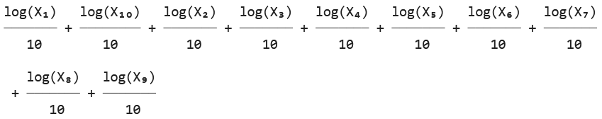
log_X = np.log(X)
gamma_hat = np.mean(log_X)
print(f"観測(ランダム)データからの最尤推定量 gamma_hat: {gamma_hat}")観測(ランダム)データからの最尤推定量 gamma_hat: 0.49849744820263612022 Q4(2)
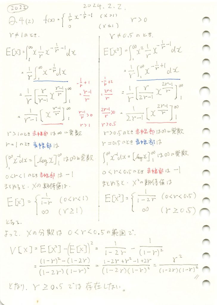
とある分布の期待値と分散を求めました。
コード
数式を使った計算
# 2022 Q4(2)  2024.8.9

from sympy import init_printing
import sympy as sp

# これでTexの表示ができる
init_printing()

# シンボリック変数の定義
x, gamma = sp.symbols('x gamma', positive=True)

# 確率密度関数 f(x) の定義
f_x = (1/gamma) * x**(-(1/gamma + 1))

# 期待値 E[X] の計算
E_X = sp.integrate(x * f_x, (x, 1, sp.oo))
E_X_simplified = sp.simplify(E_X)

# E[X^2] の計算
E_X2 = sp.integrate(x**2 * f_x, (x, 1, sp.oo))
E_X2_simplified = sp.simplify(E_X2)

# 分散 V[X] の計算
V_X = E_X2_simplified - E_X_simplified**2

# 分散をさらに簡略化
V_X_simplified = sp.simplify(V_X)
V_X_factored = sp.factor(V_X_simplified)

# 結果を表示
E_X_simplified,E_X2_simplified,V_X_simplified,V_X_factored
シミュレーションによる計算
# 2022 Q4(2)  2024.8.9

import numpy as np
import scipy.integrate as integrate

# パラメータの設定
gamma = 0.3  # 例として γ = 0.5 を設定
num_samples = 1000000  # サンプル数

# 確率密度関数 f(x) の定義
def pdf(x, gamma):
    return (1/gamma) * x**(-(1/gamma + 1))

# 理論的な期待値 E[X] の計算
def theoretical_expected_value(gamma):
    if gamma <= 0 or gamma >= 1:
        return np.inf
    else:
        result, _ = integrate.quad(lambda x: x * pdf(x, gamma), 1, np.inf)
        return result

# 理論的な分散 V[X] の計算
def theoretical_variance(gamma):
    if gamma <= 0 or gamma >= 0.5:
        return np.inf
    else:
        E_X = theoretical_expected_value(gamma)
        E_X2, _ = integrate.quad(lambda x: x**2 * pdf(x, gamma), 1, np.inf)
        return E_X2 - E_X**2

# シミュレーションによる確率変数 X のサンプリング
samples = (np.random.uniform(size=num_samples))**(-gamma)

# シミュレーションによる期待値 E[X] の推定
E_X_simulation = np.mean(samples)

# シミュレーションによる分散 V[X] の推定
V_X_simulation = np.var(samples)

# 理論値の計算
E_X_theoretical = theoretical_expected_value(gamma)
V_X_theoretical = theoretical_variance(gamma)

# 結果の表示
print(f"シミュレーションによる期待値 E[X]: {E_X_simulation}")
print(f"理論的な期待値 E[X]: {E_X_theoretical}")
print(f"シミュレーションによる分散 V[X]: {V_X_simulation}")
print(f"理論的な分散 V[X]: {V_X_theoretical}")
シミュレーションによる期待値 E[X]: 1.4284089260116615
理論的な期待値 E[X]: 1.4285714285714284
シミュレーションによる分散 V[X]: 0.4593987557711114
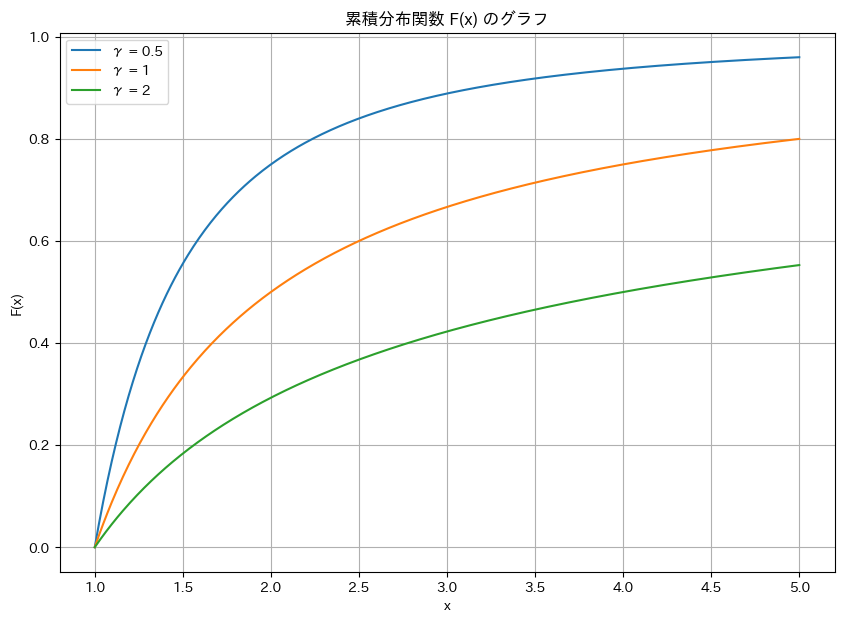
理論的な分散 V[X]: 0.459183673469389042022 Q4(1)
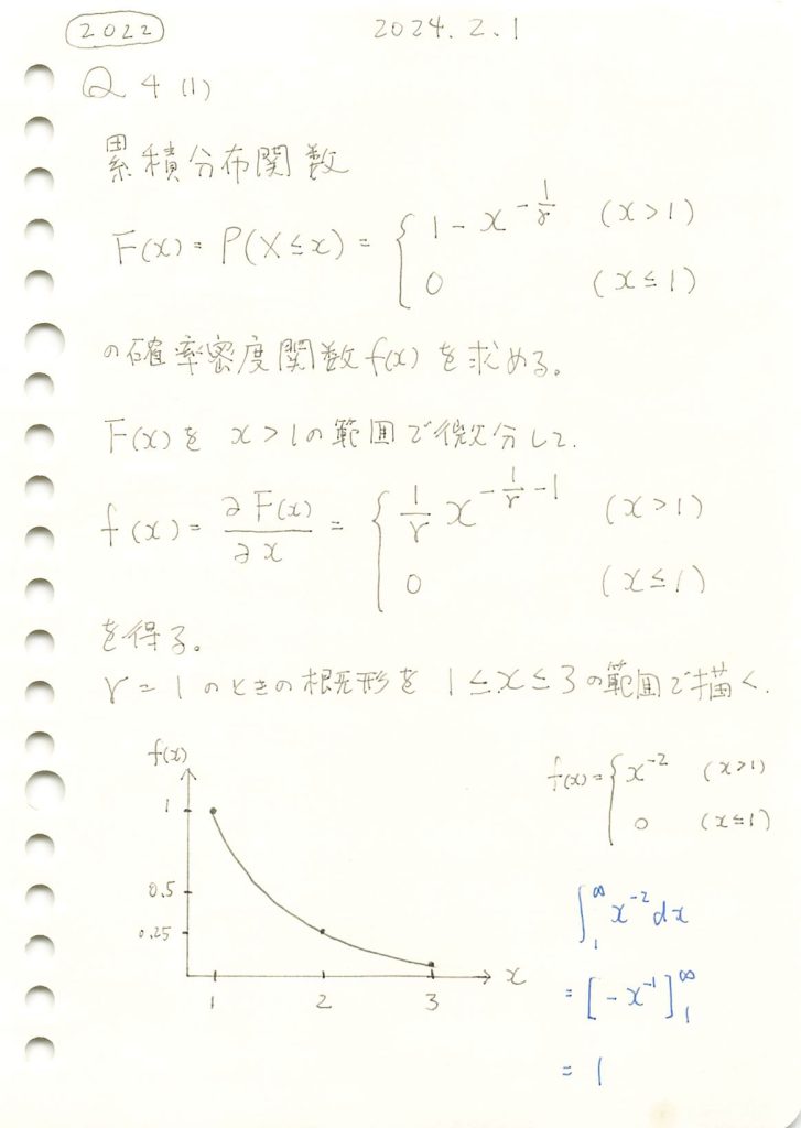
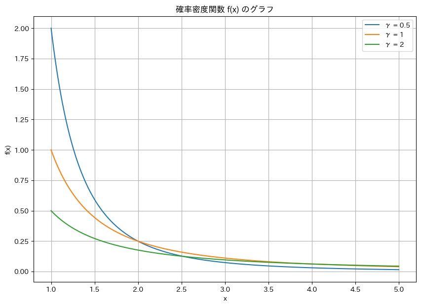
ある累積分布関数から確率密度関数を導いてグラフを描画しました。
コード
確率密度関数 f(x) の描画
# 2022 Q4(1)  2024.8.8

import numpy as np
import matplotlib.pyplot as plt

def probability_density_function(x, gamma):
    if x <= 1:
        return 0
    else:
        return (1/gamma) * x**(-1/gamma-1)

# 配列のγ値に対するベクトル化された関数
def f_array(x, gammas):
    y_values = np.zeros((len(gammas), len(x)))
    for i, gamma in enumerate(gammas):
        y_values[i] = [probability_density_function(xi, gamma) for xi in x]
    return y_values

x_values = np.linspace(1.00001, 5, 500)
gammas = [0.5, 1, 2]
y_values_pdf_array = f_array(x_values, gammas)

plt.figure(figsize=(10, 7))

for i, gamma in enumerate(gammas):
    plt.plot(x_values, y_values_pdf_array[i], label=f"γ = {gamma}")

plt.title("確率密度関数 f(x) のグラフ")
plt.xlabel("x")
plt.ylabel("f(x)")
plt.grid(True)
plt.legend()
plt.show()
累積分布関数 F(x) の描画
# 2022 Q4(1)  2024.8.8

import numpy as np
import matplotlib.pyplot as plt

# 累積分布関数を定義
def F(x, gamma):
    if x <= 1:
        return 0
    else:
        return 1 - x**(-1/gamma)

# 配列のγ値に対するベクトル化された関数
def F_array(x, gammas):
    y_values = np.zeros((len(gammas), len(x)))
    for i, gamma in enumerate(gammas):
        y_values[i] = [F(xi, gamma) for xi in x]
    return y_values

x_values = np.linspace(1, 5, 500)
gammas = [0.5, 1, 2]
y_values_array = F_array(x_values, gammas)

plt.figure(figsize=(10, 7))

for i, gamma in enumerate(gammas):
    plt.plot(x_values, y_values_array[i], label=f"γ = {gamma}")

plt.title("累積分布関数 F(x) のグラフ")
plt.xlabel("x")
plt.ylabel("F(x)")
plt.grid(True)
plt.legend()
plt.show()