2017 Q4(4)
線形関係のある確率変数の条件付き確率分布を求めました。
コード
X|Z=zが に従うかシミュレーションし確かめます。
# 2017 Q4(4)  2024.11.7

import numpy as np
import matplotlib.pyplot as plt
from scipy.stats import norm

# 定数の設定
a = 1
k = 2
num_samples = 1000000
z_fixed = 3  # 条件として与える Z の値

# シミュレーション
Y = np.random.normal(0, 1, num_samples)
X = np.random.normal(0, 1, num_samples)
Z = a + k * X + Y

# Z = z_fixed に条件を付けた X の分布を抽出
X_given_Z = (X[np.abs(Z - z_fixed) < 0.05])

# 理論値の計算
mean_conditional = (k / (k**2 + 1)) * (z_fixed - a)
std_dev_conditional = np.sqrt(1 / (k**2 + 1))

# シミュレーションによる値の計算
mean_simulation = np.mean(X_given_Z)
std_dev_simulation = np.std(X_given_Z)

# 理論値とシミュレーション値を出力
print(f"理論上の期待値 (X | Z = {z_fixed}): {mean_conditional}")
print(f"シミュレーションによる期待値: {mean_simulation}")
print(f"理論上の標準偏差: {std_dev_conditional}")
print(f"シミュレーションによる標準偏差: {std_dev_simulation}")

# 条件付き分布のヒストグラム
plt.hist(X_given_Z, bins=50, density=True, alpha=0.6, color='b', label=f"シミュレーション X | Z = {z_fixed}")

# 理論分布をプロット
x_vals = np.linspace(min(X_given_Z), max(X_given_Z), 100)
plt.plot(x_vals, norm.pdf(x_vals, mean_conditional, std_dev_conditional), 'r', label="理論分布")

# グラフの装飾
plt.title(f"条件付き分布 X | Z = {z_fixed}")
plt.xlabel("X の値")
plt.ylabel("密度")
plt.legend()
plt.show()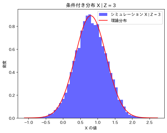
X|Z=zはに従うことが確認できました。
2017 Q4(1)(2)(3)
線形関係のある確率変数との相関係数や条件付き確率分布を求めました。
コード
(1) Zが に従うかシミュレーションし確かめます。
# 2017 Q4(1)  2024.11.6

import numpy as np
import matplotlib.pyplot as plt
from scipy.stats import norm

# 定数の設定
a = 1
k = 2
num_samples = 10000

# シミュレーション
X = np.random.normal(0, 1, num_samples)
Y = np.random.normal(0, 1, num_samples)
Z = a + k * X + Y

# 理論値の計算
mean_theory = a
std_dev_theory = np.sqrt(k**2 + 1)

# シミュレーションによる値の計算
mean_simulation = np.mean(Z)
std_dev_simulation = np.std(Z)

# 理論値とシミュレーションによる値の表示
print(f"理論上の期待値: {mean_theory}")
print(f"シミュレーションによる期待値: {mean_simulation}")
print(f"理論上の標準偏差: {std_dev_theory}")
print(f"シミュレーションによる標準偏差: {std_dev_simulation}")

# ヒストグラムのプロット
plt.hist(Z, bins=50, density=True, alpha=0.6, color='b', label="シミュレーションによる Z の分布")

# 理論分布のプロット
x_vals = np.linspace(min(Z), max(Z), 100)
plt.plot(x_vals, norm.pdf(x_vals, mean_theory, std_dev_theory), 'r', label="理論分布 N(a, k^2 + 1)")

# グラフのラベル
plt.title("Z の分布")
plt.xlabel("Z の値")
plt.ylabel("密度")
plt.legend()
plt.show()
理論上の期待値: 1
シミュレーションによる期待値: 0.9814460670948696
理論上の標準偏差: 2.23606797749979
シミュレーションによる標準偏差: 2.2474915102454482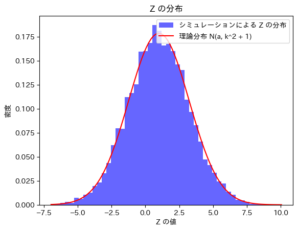
Zはに従うことが確認できました。
(2) 次に、XとZの相関係数をシミュレーションにより求めます。
# 2017 Q4(2)  2024.11.6

import numpy as np
import matplotlib.pyplot as plt

# 定数の設定
a = 1
k = 2
num_samples = 10000

# シミュレーション
X = np.random.normal(0, 1, num_samples)
Y = np.random.normal(0, 1, num_samples)
Z = a + k * X + Y

# 理論的な相関係数の計算
correlation_theory = k / np.sqrt(k**2 + 1)

# シミュレーションによる相関係数の計算
correlation_simulated = np.corrcoef(X, Z)[0, 1]

# 理論値とシミュレーションによる相関係数の表示
print(f"理論上の相関係数: {correlation_theory}")
print(f"シミュレーションによる相関係数: {correlation_simulated}")

# 相関係数の視覚化のための散布図のプロット
plt.figure(figsize=(8, 6))
plt.scatter(X, Z, alpha=0.5, s=10, label="X と Z の散布図")
plt.title("X と Z の相関関係")
plt.xlabel("X の値")
plt.ylabel("Z の値")
plt.legend()
plt.show()
理論上の相関係数: 0.8944271909999159
シミュレーションによる相関係数: 0.8943931884333798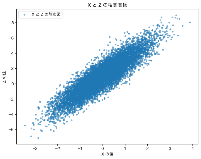
XとZの相関係数は理論値と一致しました。
(3) 次に、Z|X=xがN(a+kx,1)に従うかシミュレーションし確かめます。
# 2017 Q4(3)  2024.11.6

import numpy as np
import matplotlib.pyplot as plt
from scipy.stats import norm

# 定数の設定
a = 1
k = 2
num_samples = 10000
x_fixed = 0.5  # 条件として与える X の値

# シミュレーション
Z_given_X = a + k * x_fixed + np.random.normal(0, 1, num_samples)

# 理論値の計算
mean_conditional = a + k * x_fixed
std_dev_conditional = 1  # 分散が 1 であるため

# シミュレーションによる値の計算
mean_simulation = np.mean(Z_given_X)
std_dev_simulation = np.std(Z_given_X)

# 理論値とシミュレーションによる値の表示
print(f"理論上の期待値 (Z | X = {x_fixed}): {mean_conditional}")
print(f"シミュレーションによる期待値: {mean_simulation}")
print(f"理論上の標準偏差: {std_dev_conditional}")
print(f"シミュレーションによる標準偏差: {std_dev_simulation}")

# 条件付き分布のヒストグラムのプロット
plt.hist(Z_given_X, bins=50, density=True, alpha=0.6, color='g', label=f"シミュレーションによる Z | X = {x_fixed} の分布")

# 理論分布のプロット
z_vals = np.linspace(min(Z_given_X), max(Z_given_X), 100)
plt.plot(z_vals, norm.pdf(z_vals, mean_conditional, std_dev_conditional), 'r', label="理論分布 N(a + kx, 1)")

# グラフの装飾
plt.title(f"条件付き分布 Z | X = {x_fixed}")
plt.xlabel("Z の値")
plt.ylabel("密度")
plt.legend()
plt.show()
理論上の期待値 (Z | X = 0.5): 2.0
シミュレーションによる期待値: 1.978029240745398
理論上の標準偏差: 1
シミュレーションによる標準偏差: 1.0089203051741882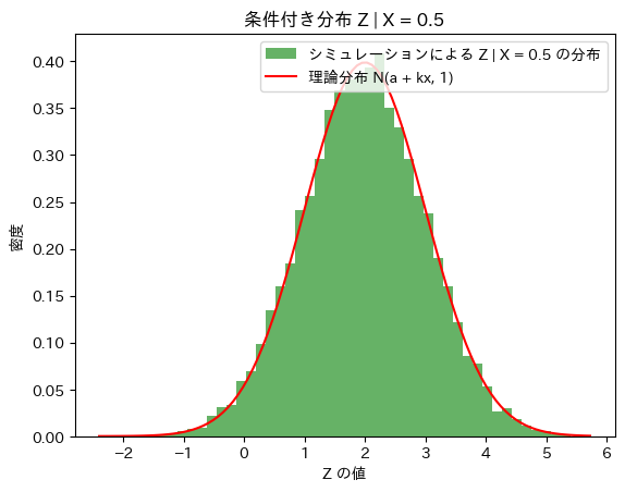
Z|X=xはN(a+kx,1)に従うことが確認できました。
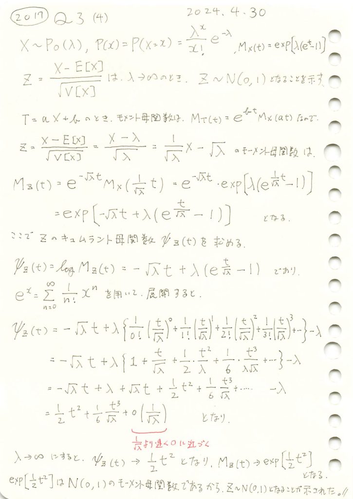
2017 Q3(4)
標準化されたポアソン分布はパラメータλを∞に近づけると標準正規分布に収束することを示しました。
コード
λを変化させて標準化されたポアソン分布Zの分布をシミュレーションにより確認してみます。
# 2017 Q3(4)  2024.11.05

import numpy as np
import matplotlib.pyplot as plt
from scipy.stats import norm

# パラメータ設定
lambda_values = [10, 20, 50, 100]
sample_size = 10000  # サンプルサイズ

# 標準正規分布の理論値
z_values = np.linspace(-4, 4, 100)
normal_pdf = norm.pdf(z_values, 0, 1)

# 2x2 のグリッドでプロット
fig, axes = plt.subplots(2, 2, figsize=(12, 10))
axes = axes.ravel()

# 各 λ に対してヒストグラムをプロット
for i, lambda_val in enumerate(lambda_values):
    # ポアソン分布からサンプルを生成し、標準化
    X_samples = np.random.poisson(lambda_val, sample_size)
    Z_samples = (X_samples - lambda_val) / np.sqrt(lambda_val)

    # 各 λ に対応するサブプロットでヒストグラムを描画
    axes[i].hist(Z_samples, bins=100, density=True, alpha=0.5, color='orange', label=f"λ = {lambda_val}")
    axes[i].plot(z_values, normal_pdf, color="red", linestyle="--", label="標準正規分布 N(0, 1)")

    # グラフのカスタマイズ
    axes[i].set_ylim(0, 1.8)
    axes[i].set_xlabel("標準化変量 Z")
    axes[i].set_ylabel("確率密度")
    axes[i].set_title(f"標準化されたポアソン分布 (λ = {lambda_val})")
    axes[i].legend()
    axes[i].grid(True)

# レイアウト調整
plt.tight_layout()
plt.show()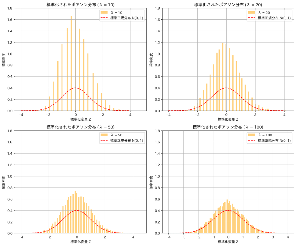
λ が増加するにつれて、標準化されたポアソン分布 Z の分布が標準正規分布に近づくことが確認できました。
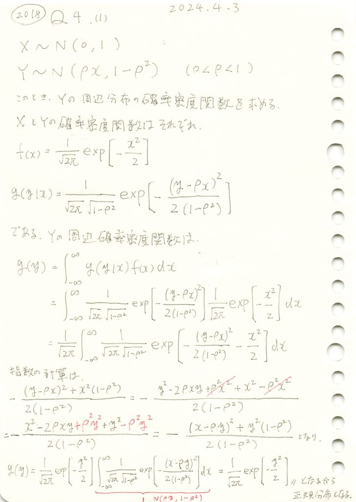
2018 Q4(1)
条件付きの正規分布の周辺確率密度関数を求めました。
コード
条件付き分布Y|X=x を生成し、Yの周辺分布が標準正規分布に従うかシミュレーションしてみます。
# 2018 Q4(1)  2024.10.18

import numpy as np
import matplotlib.pyplot as plt
from scipy.stats import norm

# パラメータ設定
rho = 0.7  # 相関係数

# サンプルサイズ
n_samples = 10000

#Xを標準正規分布からサンプル
X = np.random.normal(0, 1, n_samples)

#Y|X=x に基づいてYを生成
Y = np.random.normal(rho * X, np.sqrt(1 - rho**2))

#Yのヒストグラムを描画
plt.hist(Y, bins=50, density=True, alpha=0.6, color='g', label='シミュレーションされた Y')

# 理論的な標準正規分布N(0,1)の曲線を重ねる
x_vals = np.linspace(-4, 4, 1000)
plt.plot(x_vals, norm.pdf(x_vals, 0, 1), 'r-', lw=2, label='理論分布 N(0,1)')

# ラベルを描画
plt.title('シミュレーションされた Y と理論分布 N(0,1) の比較')
plt.xlabel('Y')
plt.ylabel('確率密度')
plt.legend()

# グラフを表示
plt.show()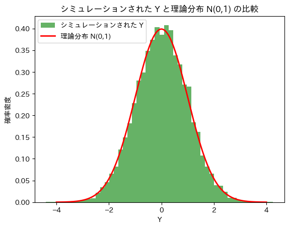
Yは標準正規分布に従うことが確認できました。
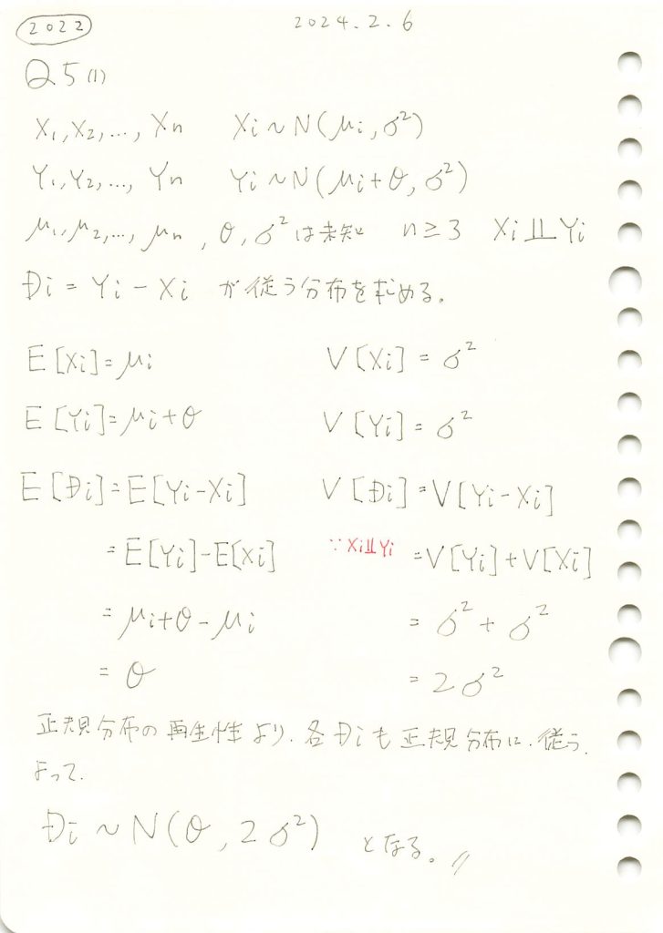
2022 Q5(1)
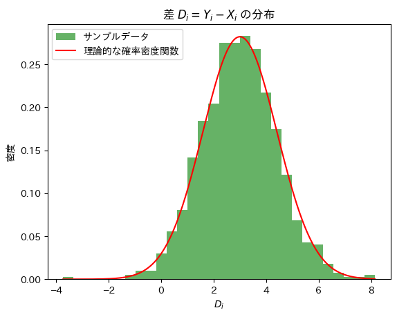
正規分布の差の分布を求める問題をやりました。
コード
シミュレーションによる計算
# 2022 Q4(5)  2024.8.13

import numpy as np
import matplotlib.pyplot as plt
import scipy.stats as stats

# パラメータの設定
mu_i = 5.0  # 平均値 mu_i
theta = 3.0  # シフトパラメータ θ
sigma = 1.0  # 標準偏差 σ
n = 1000  # サンプル数

# X_i と Y_i のサンプル生成
X_i = np.random.normal(mu_i, sigma, n)
Y_i = np.random.normal(mu_i + theta, sigma, n)

# D_i の計算
D_i = Y_i - X_i

# シミュレーション結果の平均と分散を計算
mean_simulation = np.mean(D_i)
variance_simulation = np.var(D_i)

# 理論上の平均と分散
mean_theoretical = theta
variance_theoretical = 2 * sigma**2

# 結果の表示
print(f"シミュレーション結果: 平均 = {mean_simulation}, 分散 = {variance_simulation}")
print(f"理論値: 平均 = {mean_theoretical}, 分散 = {variance_theoretical}")

# サンプルのヒストグラムを作成
plt.hist(D_i, bins=30, density=True, alpha=0.6, color='g', label='サンプルデータ')

# 理論上の分布を重ねる
x = np.linspace(min(D_i), max(D_i), 1000)
plt.plot(x, stats.norm.pdf(x, mean_theoretical, np.sqrt(variance_theoretical)), 'r', label='理論的な確率密度関数')

plt.title("差 $D_i = Y_i - X_i$ の分布")
plt.xlabel("$D_i$")
plt.ylabel("密度")
plt.legend()
plt.show()
シミュレーション結果: 平均 = 2.975536685240219, 分散 = 2.005575154363111
理論値: 平均 = 3.0, 分散 = 2.0