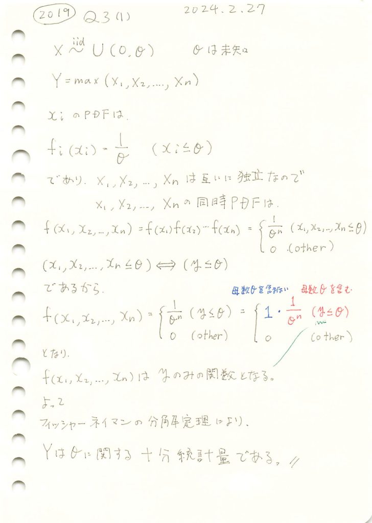
一様分布に於いて最大値が十分統計量であることを示しました。
コード
一様分布の最大値Yを元に、不偏推定量 を計算します。
import numpy as np
import matplotlib.pyplot as plt

# シミュレーションパラメータ
n = 10  # サンプルサイズ
theta_true = 10  # 真のθ
num_simulations = 1000  # シミュレーション回数

# θの推定値を格納するリスト
theta_estimates = []

# シミュレーション開始
for _ in range(num_simulations):
    # (0, theta_true) の一様分布からn個のサンプルを生成
    samples = np.random.uniform(0, theta_true, n)

    # 最大値 Y = max(X_1, ..., X_n)
    Y = np.max(samples)

    # Y から θ を推定 (最大値を使って推定)
    theta_hat = Y * (n / (n - 1))  # 推定式: Y * n / (n-1)

    # 推定されたθをリストに保存
    theta_estimates.append(theta_hat)

# θの推定値の平均を計算
theta_mean = np.mean(theta_estimates)

# 推定結果をヒストグラムで表示
plt.hist(theta_estimates, bins=30, alpha=0.7, color='blue', edgecolor='black', label='推定されたθ')
plt.axvline(x=theta_true, color='red', linestyle='--', label=f'真のθ = {theta_true}')
plt.axvline(x=theta_mean, color='green', linestyle='--', label=f'推定されたθの平均 = {theta_mean:.2f}')
plt.title(f'Y (最大値) に基づく θ の推定値のヒストグラム ({n} サンプル)')
plt.xlabel('推定された θ')
plt.ylabel('頻度')
plt.legend()
plt.show()

# 推定結果をテキストで表示
print(f'真のθ: {theta_true}')
print(f'推定されたθの平均: {theta_mean:.2f}')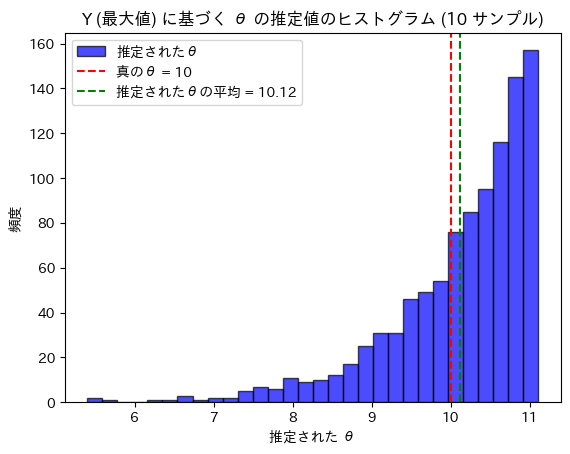
真のθ: 10
推定されたθの平均: 10.12
推定されたθは真のθに近い値を取りました。最大値Yだけを用いてθが正確に推定できたので、Yはθに関する十分統計量であることが確認できました。