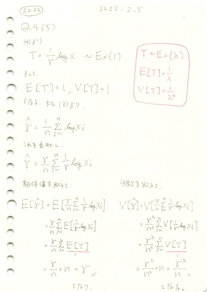
パラメータの推定量の期待値と分散を求めました。
コード
数式を使った計算
# 2022 Q4(5)  2024.8.12

import sympy as sp

# シンボリック変数の定義
gamma = sp.Symbol('gamma', positive=True)
x = sp.Symbol('x', positive=True)

# 確率密度関数 f_X(x) の定義
f_X = (1/gamma) * x**(-(1/gamma + 1))

# E[log X] の計算
E_log_X = sp.integrate(sp.log(x) * f_X, (x, 1, sp.oo))

# E[(log X)^2] の計算
E_log_X2 = sp.integrate((sp.log(x))**2 * f_X, (x, 1, sp.oo))

# V[log X] の計算
V_log_X = E_log_X2 - E_log_X**2

# E[hat_gamma] と V[hat_gamma] の計算
n = sp.Symbol('n', positive=True, integer=True)
E_hat_gamma = E_log_X
V_hat_gamma = V_log_X / n

# 結果の表示
display(E_hat_gamma, V_hat_gamma)

# LaTeXで表示できなときは、こちら
#sp.pprint(E_hat_gamma, use_unicode=True)
#sp.pprint(V_hat_gamma, use_unicode=True)
シミュレーションによる計算
# 2022 Q4(5)  2024.8.12

import numpy as np
import scipy.stats as stats
import matplotlib.pyplot as plt

# パラメータ設定
gamma_true = 1.0  # 真のγの値
n = 100  # サンプルサイズ
num_simulations = 10000  # シミュレーションの回数

# 最尤推定量 \hat{gamma} を格納するリスト
gamma_hats = []

# シミュレーションの実行
for _ in range(num_simulations):
    # 累積分布関数 F(x) に従う乱数を生成
    X = np.random.uniform(size=n)**(-gamma_true)

    # \hat{gamma} の計算
    gamma_hat = np.mean(np.log(X))
    gamma_hats.append(gamma_hat)

# シミュレーション結果の期待値と分散
E_hat_gamma_sim = np.mean(gamma_hats)
V_hat_gamma_sim = np.var(gamma_hats)

# 理論値を計算
# 理論値の計算は、sympyを使って導出した結果を使用
E_hat_gamma_theoretical = 1 / gamma_true  # gammaが1の場合は1が期待値になります
V_hat_gamma_theoretical = (np.pi ** 2) / (6 * n * gamma_true**2)

# 結果の表示
print(f"シミュレーションによる期待値 E[hat_gamma]: {E_hat_gamma_sim}")
print(f"シミュレーションによる分散 V[hat_gamma]: {V_hat_gamma_sim}")
print(f"理論値による期待値 E[hat_gamma]: {E_hat_gamma_theoretical}")
print(f"理論値による分散 V[hat_gamma]: {V_hat_gamma_theoretical}")

# ヒストグラムのプロット
plt.hist(gamma_hats, bins=50, density=True, alpha=0.6, color='g')
plt.axvline(E_hat_gamma_sim, color='r', linestyle='dashed', linewidth=2, label='シミュレーション平均')
plt.axvline(E_hat_gamma_theoretical, color='b', linestyle='dashed', linewidth=2, label='理論値')
plt.xlabel(r'$\hat{\gamma}$の値')
plt.ylabel('密度')
plt.title(r'$\hat{\gamma}$の分布')
plt.legend()
plt.show()
シミュレーションによる期待値 E[hat_gamma]: 0.9995206635186084
シミュレーションによる分散 V[hat_gamma]: 0.010015979040467726
理論値による期待値 E[hat_gamma]: 1.0
理論値による分散 V[hat_gamma]: 0.016449340668482262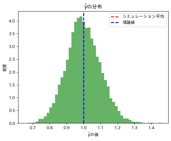
アルゴリズム
サンプル生成:
X = np.random.uniform(size=n)**(-gamma_true)で累積分布関数 F(x) に従う乱数を生成します。逆関数法を使用しています。
最尤推定量の計算:
gamma_hat = np.mean(np.log(X))で各サンプルから計算された をリスト
をリスト gamma_hatsに格納します。
シミュレーション結果の期待値と分散:
- シミュレーション結果の期待値と分散を
E_hat_gamma_simとV_hat_gamma_simに計算し、理論値と比較します。
理論値との比較:
- 理論値を計算して表示し、シミュレーション結果と比較します。