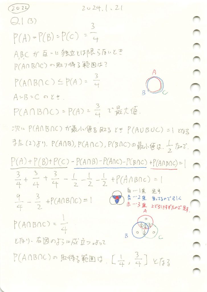
2022 Q1(3)
事象A,B,Cが独立とは限らない場合のP(A∩B∩C)の取り得る範囲を求めました。
コード
### 2022 Q1(3)   2024.7.27

import itertools

def generate_combinations(n, k):
    base_list = [1] * k + [0] * (n - k)
    all_combinations = set(itertools.permutations(base_list))
    return list(all_combinations)

def calculate_intersection(A, B, C):
    return np.mean(np.array(A) & np.array(B) & np.array(C))

def find_min_max_intersection(n, k):
    all_combinations = generate_combinations(n, k)
    min_intersection = 1.0
    max_intersection = 0.0

    for A in all_combinations:
        for B in all_combinations:
            for C in all_combinations:
                intersection_ratio = calculate_intersection(A, B, C)
                if intersection_ratio < min_intersection:
                    min_intersection = intersection_ratio
                if intersection_ratio > max_intersection:
                    max_intersection = intersection_ratio

    return min_intersection, max_intersection

# パラメータを設定
n = 8
k = 6

# 最小値と最大値を計算
min_intersection, max_intersection = find_min_max_intersection(n, k)

min_intersection, max_intersection
(0.25, 0.75)アルゴリズム
- 組み合わせの生成
- 配列の長さ
nを8、1の数kを6と設定する。 - 配列
11111100を作成し、itertools.permutationsを使ってすべての並べ替えを生成する。
- 配列の長さ
- 交差部分の確率計算
- すべての組み合わせに対して、配列
A,B,Cを選ぶ。 - 例えば、
A = 11111100,B = 11011110,C = 11101110の場合、交差部分A & B & Cは11001100となる。これにより、確率は となる。
となる。
- すべての組み合わせに対して、配列
- 最小値と最大値の取得
- すべての組み合わせに対して計算した確率を比較し、最小値と最大値を更新する。
- 最終的に、最小値と最大値を返す。
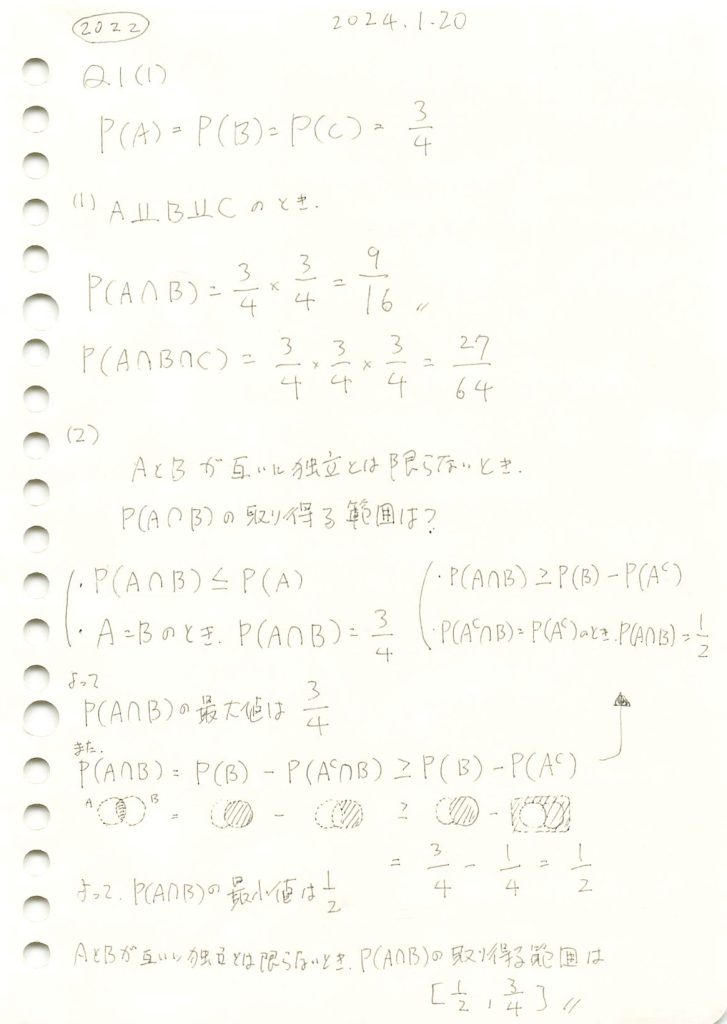
2022 Q1(1)(2)
事象A,Bが独立なときと、そうとは限らない場合の確率の取り得る範囲の計算をしました。
(1)コード
### 2022 Q1(1)   2024.7.26

import numpy as np

# シミュレーションの回数
num_simulations = 1000000

# 与えられた確率
prob = 3/4

# 事象 A, B, C をシミュレーション
A = np.random.rand(num_simulations) < prob
B = np.random.rand(num_simulations) < prob
C = np.random.rand(num_simulations) < prob

# 交差確率の計算
P_A_and_B = np.mean(A & B)
P_A_and_B_and_C = np.mean(A & B & C)

P_A_and_B, P_A_and_B_and_C
(0.56311, 0.422594)#検算
9/16,27/64(0.5625, 0.421875)(2)コード
### 2022 Q1(2)   2024.7.26

import numpy as np

def simulate_overlap_with_fixed_true(correlation):
    P_A = 3/4
    P_B = 3/4
    num_elements = 1000
    num_true_A = int(P_A * num_elements)
    num_true_B = int(P_B * num_elements)

    # A と B の配列を生成し、3/4がtrueになるように設定
    A = np.zeros(num_elements, dtype=bool)
    A[:num_true_A] = True
    np.random.shuffle(A)

    B = np.zeros(num_elements, dtype=bool)
    B[:num_true_B] = True
    np.random.shuffle(B)

    if correlation == 'positive':
        # 正の相関を持たせるために、スワップを行う
        A1_B0_indices = np.where(A & ~B)[0]
        A0_B1_indices = np.where(~A & B)[0]

        min_len = min(len(A1_B0_indices), len(A0_B1_indices))
        for i in range(min_len):
            B[A1_B0_indices[i]], B[A0_B1_indices[i]] = B[A0_B1_indices[i]], B[A1_B0_indices[i]]

    elif correlation == 'negative':
        # 負の相関を持たせるために、スワップを行う
        A1_B1_indices = np.where(A & B)[0]
        A0_B0_indices = np.where(~A & ~B)[0]

        min_len = min(len(A1_B1_indices), len(A0_B0_indices))
        for i in range(min_len):
            B[A1_B1_indices[i]], B[A0_B0_indices[i]] = B[A0_B0_indices[i]], B[A1_B1_indices[i]]

    else:
        raise ValueError("Invalid correlation type")

    # 重なりの割合を計算
    overlap_ratio = np.mean(A & B)

    return overlap_ratio

# 正の相関の場合
overlap_positive = simulate_overlap_with_fixed_true('positive')

# 負の相関の場合
overlap_negative = simulate_overlap_with_fixed_true('negative')

overlap_positive, overlap_negative
(0.75, 0.5)アルゴリズム
- パラメータの設定
- 事象 (A) の発生確率 (P_A) を設定する(ここでは 3/4)。
- 事象 (B) の発生確率 (P_B) を設定する(ここでは 3/4)。
- 配列の要素数 (num_elements) を設定する(ここでは 1000)。
- シミュレーションの回数 (num_simulations) を設定する(ここでは 1000)。
- 配列の初期化
- 配列 (A) と (B) をそれぞれ3/4がtrueになるように生成する。
- 配列 (A) に対して、最初の (num_true_A) 個を true に設定し、残りを false に設定する。その後、配列をシャッフルする。
- 配列 (B) に対しても同様の処理を行う。
- 相関の付与
- 正の相関を持たせる場合:
- 配列 (A) と (B) の要素をスワップして、 (A = 1, B = 0) と (A = 0, B = 1) の組を見つけたら、これらをスワップして値を揃える。
- 負の相関を持たせる場合:
- 配列 (A) と (B) の要素をスワップして、 (A = 1, B = 1) と (A = 0, B = 0) の組を見つけたら、これらをスワップして値が揃わないようにする。
- 重なりの割合の計算
- 配列 (A) と (B) の共通部分(重なり部分)を計算し、その割合を求める。
- 結果の記録
- 重なりの割合をリストに記録する。
- シミュレーション回数分、上記のステップを繰り返す。
- 最小値と最大値の取得
- 重なりの割合のリストから、最小値と最大値を取得する。
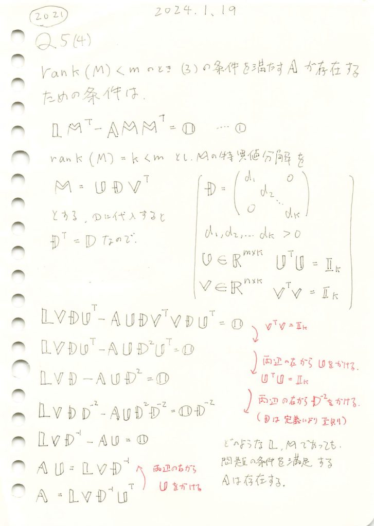
2021 Q5(4)
特異値分解を用いてMが行フルランクでない場合に先の問の条件を満たすAが存在するか論ずる問題をやりました。
コード
M行列のrank(M)を5~1に変化させて、A行列を特異値分解により計算し、 の変化を確認します。
# 2021 Q5(4)  2024.9.8

import numpy as np
import matplotlib.pyplot as plt
import seaborn as sns

# l, n を定義
l = 5  # Lの行数
n = 5  # LとMの列数 (xの次元)

# 再現性のために乱数のシードを固定
np.random.seed(43)

# L行列を生成。-10から10の間の整数でランダムなL行列
L = np.random.randint(-10, 11, size=(l, n))

# N(0, 1) に従う乱数ベクトル x を生成 (サンプル数を1000000に設定)
sample_size = 1000000
x = np.random.randn(n, sample_size)

# グラフの準備(2行3列のグリッドに5つのヒートマップを描画するので、6個目は空白にする)
fig, axs = plt.subplots(2, 3, figsize=(15, 10))  # 2行3列のサブプロットを作成
axs = axs.flatten()  # インデックス操作を簡単にするためフラット化

# m を 5 から 1 まで変化させて実験
for idx, m in enumerate(range(5, 0, -1)):
    # M行列を生成。-10から10の間の整数でランダムなM行列
    while True:
        M = np.random.randint(-10, 11, size=(m, n))
        if np.linalg.matrix_rank(M) == m:  # Mが行フルランクかどうかを判定
            break

    # Mの特異値分解: M = U * D * V^T
    U, D, VT = np.linalg.svd(M)

    # 特異値の逆数を作成 (ゼロ除算を回避)
    D_inv = np.diag([1/d if d > 1e-10 else 0 for d in D])  # Dの逆行列。特異値が0のところは無視

    # L の形状に応じて A を計算
    A = np.dot(np.dot(np.dot(L, VT.T[:n, :m]), D_inv[:m, :m]), U.T[:m, :])

    # Lx, Mx, AMx を計算
    Lx = np.dot(L, x)  # lxサンプル数の行列
    Mx = np.dot(M, x)  # mxサンプル数の行列
    AMx = np.dot(A, Mx)  # AMx の計算

    # 共分散行列 Cov(Lx - AMx, Mx) を計算
    cov_matrix_Lx_AMx_Mx = np.zeros((l, m))
    for i in range(l):
        for j in range(m):
            cov_matrix_Lx_AMx_Mx[i, j] = np.cov(Lx[i, :] - AMx[i, :], Mx[j, :])[0, 1]

    # 各サブプロットにヒートマップを描画
    sns.heatmap(cov_matrix_Lx_AMx_Mx, cmap="coolwarm", annot=True, fmt=".2f", center=0, vmin=-1, vmax=1, ax=axs[idx])
    axs[idx].set_title(f'm={m}')

# 6個目のサブプロットを消す(最後の空のプロットを非表示にする)
fig.delaxes(axs[5])

# グラフを描画
plt.suptitle('共分散行列 Cov(Lx - AMx, Mx) の変化 (mの変化)', fontsize=16)
plt.tight_layout(rect=[0, 0, 1, 0.96])  # タイトルとレイアウト調整
plt.show()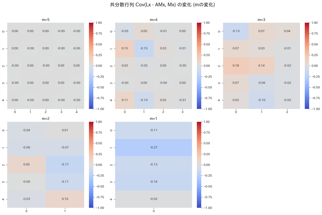
m=1~5のどのランクにおいても、A行列が見つかりはゼロ行列に近づきました。またmが減少するにつれては大きくなることを確認しました。
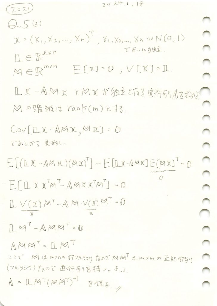
2021 Q5(3)
二つの式を互いに独立にする、実行列Aを求める問題をやりました。
コード
A行列を用いて、Lx – AMx と Mx の独立性を検証してみます。
まず、L行列とM行列を乱数で生成します。ただしM行列は行フルランクになるようします。
 も求めます。
# 2021 Q5(3)  2024.9.7

import numpy as np

# l, m, n を定義
l = 5  # Lの行数
m = 5  # Mの行数
n = 5  # LとMの列数 (xの次元)

# 再現性のために乱数のシードを固定
np.random.seed(43)

# L行列を生成。-10から10の間の整数でランダムなL行列
L = np.random.randint(-10, 11, size=(l, n))

# M行列を生成。-10から10の間の整数でランダムなM行列
# 但し、M がフルランク(ランクが n と等しい)になるまで繰り返す
while True:
    M = np.random.randint(-10, 11, size=(m, n))
    if np.linalg.matrix_rank(M) == m:  # Mが行フルランクかどうかを判定
        break

# A行列を求める: A = L * M^T * (M * M^T)^(-1)
A = np.dot(np.dot(L, M.T), np.linalg.inv(np.dot(M, M.T)))

# 結果を表示
print("L行列:\n", L)
print("\nM行列:\n", M)
print("\nA行列 (L, Mから計算):\n", A)
L行列:
[[ -6 -10 7 6 9]
[ 7 -8 4 -10 -7]
[ 8 1 -9 5 -8]
[ 1 -8 -7 -6 -6]
[ 6 2 5 -10 0]]
M行列:
[[ 6 -1 -8 6 10]
[ -6 -1 -3 10 5]
[ -2 -10 -7 -8 -1]
[ 1 6 -2 0 -3]
[ -7 9 -8 4 0]]
A行列 (L, Mから計算):
[[-0.11382722 0.14885099 -0.47741032 -2.97220233 0.34379272]
[-0.2300306 0.14696309 0.62486166 1.60321594 -1.2726385 ]
[ 0.0655719 2.52963674 1.25657509 6.68244255 -2.65929952]
[-0.16838096 0.98942126 1.29721372 2.65536098 -1.12655426]
[ 0.26046481 -1.95599245 -0.55640909 -2.20630167 0.88646572]]次に、がゼロ行列になっているか確認します
import numpy as np
import matplotlib.pyplot as plt
import seaborn as sns

# N(0, 1) に従う乱数ベクトル x を生成 (サンプル数を1000000に設定)
sample_size = 1000000
x = np.random.randn(n, sample_size)

# Lx, Mx, AMx を計算
Lx = np.dot(L, x)  # lxサンプル数の行列
Mx = np.dot(M, x)  # mxサンプル数の行列
AMx = np.dot(A, Mx)  # AMx の計算

# 共分散行列 Cov(Lx - AMx, Mx) を計算
cov_matrix_Lx_AMx_Mx = np.zeros((l, m))
for i in range(l):
    for j in range(m):
        cov_matrix_Lx_AMx_Mx[i, j] = np.cov(Lx[i, :] - AMx[i, :], Mx[j, :])[0, 1]

# ヒートマップを描画
plt.figure(figsize=(6, 6))

# 共分散行列 Cov(Lx - AMx, Mx) のヒートマップ
sns.heatmap(cov_matrix_Lx_AMx_Mx, cmap="coolwarm", annot=True, fmt=".2f", center=0, vmin=-1, vmax=1)
plt.title('共分散行列 Cov(Lx - AMx, Mx)')

plt.tight_layout()
plt.show()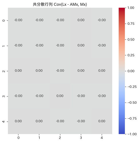
ゼロ行列になっています。検証ができました。
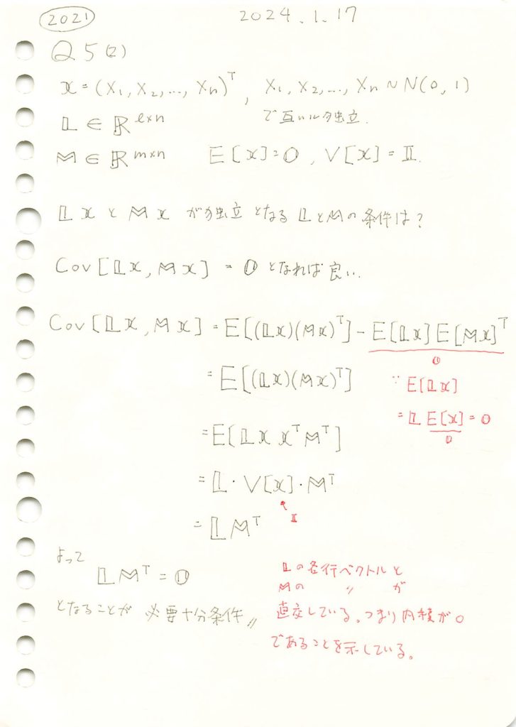
2021 Q5(2)
線形変換により得られた二つのベクトルが独立となる条件を求める問題をやりました。
コード
各行ベクトルが直交している行列LとMを生成します
# 2021 Q5(2)  2024.9.6

import numpy as np

# 乱数で4つの要素を持つ基準ベクトルを生成 (整数で0以外の値のみ)
def generate_random_integer_vector_4(n=4):
    return np.random.randint(1, 10, size=n)  # 1から9の範囲で整数を生成

# 生成した基準ベクトルを使って、並行するベクトルを生成
def generate_parallel_matrix_4(v, scale_factors):
    L = np.array([scale * v for scale in scale_factors])
    return L

# ベクトル v に直交するベクトルを生成する関数
# グラム・シュミット法を適用して、基準ベクトルに直交するベクトルを作る
def generate_orthogonal_vectors_4(v):
    orthogonal_vectors = []
    for _ in range(5):
        candidate = np.random.randint(1, 10, size=v.shape)  # 新たな候補ベクトル
        # 直交条件:v と candidate の内積が 0 になるように調整
        adjustment = np.dot(candidate, v) / np.dot(v, v)
        orthogonal_vector = candidate - adjustment * v  # 直交ベクトルにする
        orthogonal_vectors.append(orthogonal_vector)
    return np.array(orthogonal_vectors)

# 基準ベクトルを生成
v_base = generate_random_integer_vector_4()

# 基準ベクトルと並行するベクトルを5つ作る
scale_factors_5 = [1, 2, 3, 4, 5]
L_5x4 = generate_parallel_matrix_4(v_base, scale_factors_5)

# 基準ベクトルに直交するベクトルを5つ作る
M_5x4 = generate_orthogonal_vectors_4(v_base)

# 行列 L, M の表示とその積の確認
L_5x4, M_5x4, np.dot(L_5x4, M_5x4.T)  # L, M, そしてその積を表示
(array([[ 7, 1, 6, 8],
[14, 2, 12, 16],
[21, 3, 18, 24],
[28, 4, 24, 32],
[35, 5, 30, 40]]),
array([[-3.01333333, 8.42666667, -2.44 , 3.41333333],
[-1.68666667, 6.47333333, 3.84 , -2.21333333],
[ 1.28666667, 4.32666667, 0.96 , -2.38666667],
[ 1.14666667, 3.30666667, 2.84 , -3.54666667],
[-2.73333333, 4.46666667, -1.2 , 2.73333333]]),
array([[-7.10542736e-15, 7.10542736e-15, 0.00000000e+00,
-3.55271368e-15, 0.00000000e+00],
[-1.42108547e-14, 1.42108547e-14, 0.00000000e+00,
-7.10542736e-15, 0.00000000e+00],
[-2.13162821e-14, 2.13162821e-14, 7.10542736e-15,
0.00000000e+00, -7.10542736e-15],
[-2.84217094e-14, 2.84217094e-14, 0.00000000e+00,
-1.42108547e-14, 0.00000000e+00],
[-3.55271368e-14, 2.84217094e-14, 0.00000000e+00,
-2.84217094e-14, -7.10542736e-15]]))行列LとMを生成し、 を求めました。はほぼゼロ行列になっています。
LxとMxの共分散行列を求めます
# 2021 Q5(2)  2024.9.6

import numpy as np
import matplotlib.pyplot as plt
import seaborn as sns

# l, m, n を定義
l = 5  # Lの行数
m = 5  # Mの行数
n = 4  # LとMの列数 (xの次元)

# L と M を定義 (与えられた行列を使用)
L = np.array([[7, 1, 6, 8],
              [14, 2, 12, 16],
              [21, 3, 18, 24],
              [28, 4, 24, 32],
              [35, 5, 30, 40]])

M = np.array([[-3.01333333, 8.42666667, -2.44, 3.41333333],
              [-1.68666667, 6.47333333, 3.84, -2.21333333],
              [1.28666667, 4.32666667, 0.96, -2.38666667],
              [1.14666667, 3.30666667, 2.84, -3.54666667],
              [-2.73333333, 4.46666667, -1.2, 2.73333333]])

# N(0, 1) に従う乱数ベクトル x を生成 (サンプル数を10000000にする)
sample_size = 10000000
x = np.random.randn(n, sample_size)

# Lx と Mx を計算
Lx = np.dot(L, x)  # lxサンプル数の行列
Mx = np.dot(M, x)  # mxサンプル数の行列

# 共分散行列 Cov(Lx, Mx) を計算
cov_matrix = np.zeros((l, m))
for i in range(l):
    for j in range(m):
        cov_matrix[i, j] = np.cov(Lx[i, :], Mx[j, :])[0, 1]

# L * M^T の積を再計算
LM_T = np.dot(L, M.T)

# ヒートマップを描画
plt.figure(figsize=(12, 6))

# 共分散行列のヒートマップ
plt.subplot(1, 2, 1)
sns.heatmap(cov_matrix, cmap="coolwarm", annot=True, fmt=".2f", center=0, vmin=-1, vmax=1)
plt.title(f'共分散行列 Cov(Lx, Mx)')

# L * M^T のヒートマップ
plt.subplot(1, 2, 2)
sns.heatmap(LM_T, cmap="coolwarm", annot=True, fmt=".2f", center=0, vmin=-1, vmax=1)
plt.title(f'行列 L * M^T')

plt.tight_layout()
plt.show()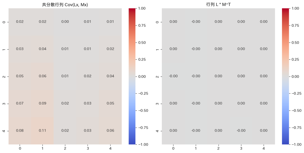
Cov(Lx,Mx)はゼロ行列に近づきます。その必要十分条件はがゼロ行列になることです。
ここで注意が必要なのは、LxとMxは確率変数から成るベクトルであり、Cov(Lx,Mx)はLxとMxのそれぞれの確率変数同士の共分散を計算し、それを行列としてまとめたものです。
2021 Q5(1)
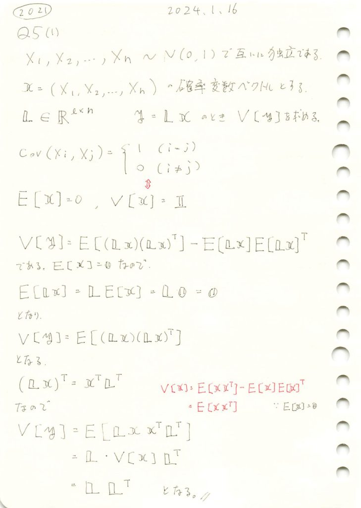
線形変換された確率変数ベクトルの分散共分散行列を求める問題をやりました。
コード
シミュレーション
乱数による分散共分散行列と、 を比較します
# 2021 Q5(1)  2024.9.4

import numpy as np
import matplotlib.pyplot as plt
import seaborn as sns

# 標準正規分布からサンプルを生成
n = 1000  # サンプル数
d = 5  # 次元数
X = np.random.randn(d, n)

# 4x5の線形変換行列 L を定義
L = np.array([[9, 7, 8, 6, 5],
              [6, 5, 4, 3, 2],
              [3, 2, 1, 9, 8],
              [8, 7, 6, 5, 0]])

# 線形変換を適用して y を計算
Y = np.dot(L, X)

# y のサンプルから分散共分散行列を推定
V_Y_estimated = np.cov(Y)

# 理論的な L・L^T と比較
V_Y_theoretical = np.dot(L, L.T)

# ヒートマップのプロット
plt.figure(figsize=(12, 6))

# 推定された分散共分散行列のヒートマップ
plt.subplot(1, 2, 1)
sns.heatmap(V_Y_estimated, annot=True, cmap="coolwarm", cbar=True)
plt.title("推定された分散共分散行列")

# 理論的な分散共分散行列のヒートマップ
plt.subplot(1, 2, 2)
sns.heatmap(V_Y_theoretical, annot=True, cmap="coolwarm", cbar=True)
plt.title("理論的な分散共分散行列")

plt.show()
同じような行列になりました。違いは乱数によるものです。
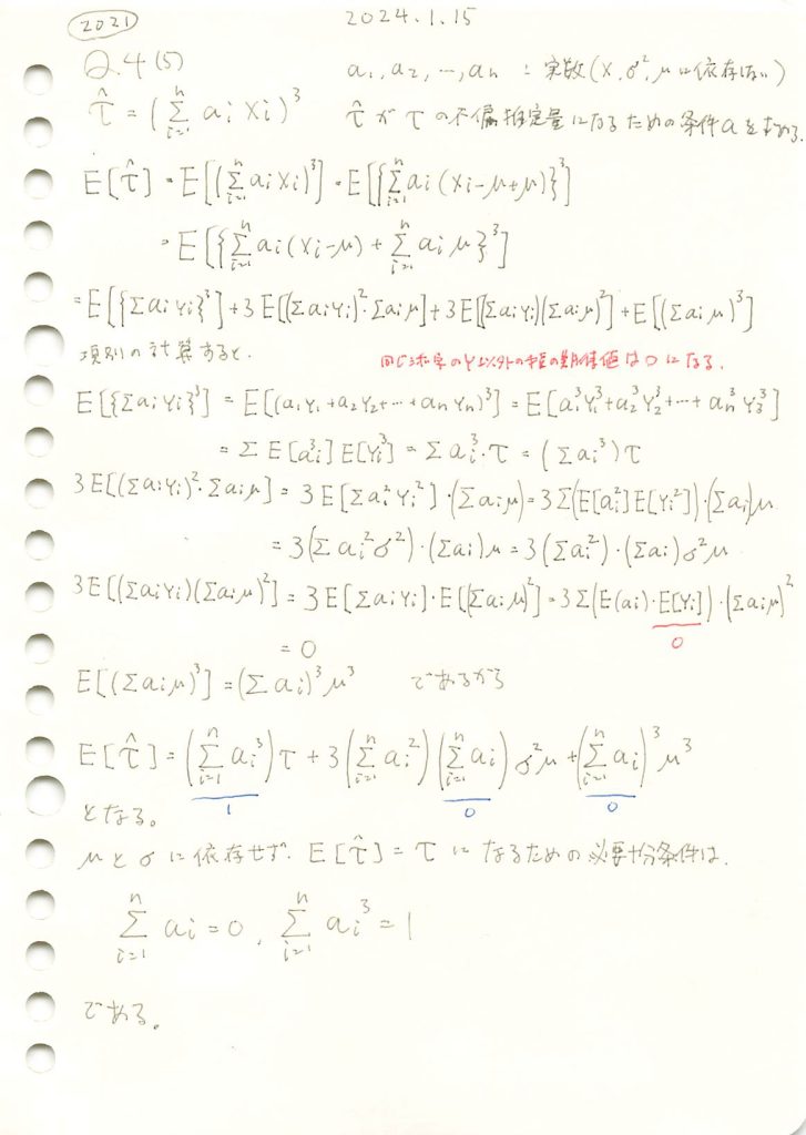
2021 Q4(5)
τハットがτの不偏推定量になるための必要十分条件を求める問題を学びました。
コード
 を満たすaiを見つける
# 2021 Q4(5)  2024.9.3

import numpy as np

def find_ai_sequence(n, tolerance=1e-6):
    while True:
        # ランダムに n 個の値を生成
        a = np.random.uniform(-1, 1, n)

        # 正の数と負の数の個数を調整
        neg_count = (n + 1) // 2  # 負の数を1つ多くする
        pos_count = n - neg_count

        a[:pos_count] = np.abs(a[:pos_count])
        a[pos_count:] = -np.abs(a[pos_count:])

        # 合計が0になるように調整
        a -= np.mean(a)

        # 条件をチェック
        sum_ai = np.sum(a)
        sum_ai_cubed = np.sum(a**3)

        if np.abs(sum_ai) < tolerance and np.abs(sum_ai_cubed - 1) < tolerance:
            return a

# パラメータの設定
n = 10  # サンプル数

# 条件を満たす a_i の数列を見つける
a = find_ai_sequence(n)

# 計算を確認
print(f"a_i の合計 (≒0): {a.sum()}")
print(f"a_i^3 の合計 (≒1): {np.sum(a ** 3)}")

# 条件を満たした a_i を表示
print("a_i の数列:")
print(a)
a_i の合計 (≒0): 6.661338147750939e-16
a_i^3 の合計 (≒1): 1.0000001485058854
a_i の数列:
[ 0.13279542 1.05885499 0.24951311 0.83492921 0.13800083 -0.71178855
-0.38213634 -0.18394766 -0.55820111 -0.5780199 ]5分ほどで見つかった
見つかったaiと指数分布に従う乱数を使って のシミュレーションしてみる
import numpy as np
import matplotlib.pyplot as plt

# すでに見つかった条件を満たす a_i を使用
a = np.array([ 0.13279542,  1.05885499,  0.24951311,  0.83492921,  0.13800083, -0.71178855,
              -0.38213634, -0.18394766, -0.55820111, -0.5780199 ])

# パラメータの設定
n = len(a)  # サンプル数(a_i の数と一致させる)
scale = 1.0  # 指数分布のスケールパラメータ
iterations = 10000  # シミュレーション回数

# シミュレーション結果を保存するリスト
tau_hat_values = []

# シミュレーションを実行
for _ in range(iterations):
    # 指数分布に従う乱数を生成
    X = np.random.exponential(scale=scale, size=n)

    # \hat{\tau} の計算
    tau_hat = np.sum(a * X) ** 3
    tau_hat_values.append(tau_hat)

# 指数分布の三次中心モーメントを計算
tau = 2 * scale**3  # 指数分布における三次中心モーメント

# シミュレーション結果の平均
simulated_mean_tau_hat = np.mean(tau_hat_values)

# 結果を表示
print(f"理論値の τ: {tau}")
print(f"シミュレーションによる τ の推定値: {simulated_mean_tau_hat}")

# 視覚化
plt.figure(figsize=(10, 6))
plt.hist(tau_hat_values, bins=50, alpha=0.75, label='シミュレーション結果')
plt.axvline(simulated_mean_tau_hat, color='red', linestyle='dashed', linewidth=2, label=f'シミュレーション平均 = {simulated_mean_tau_hat:.2f}')
plt.axvline(tau, color='blue', linestyle='dashed', linewidth=2, label=f'理論値 = {tau:.2f}')
plt.xlabel('値')
plt.ylabel('頻度')
plt.title(r"$\hat{\tau} = \left(\sum_{i=1}^{n} a_i X_i\right)^3$ の分布 (指数分布)")
plt.legend()
plt.grid(True)
plt.show()
理論値の τ: 2.0
シミュレーションによる τ の推定値: 2.0555706049874143
推定値は理論値と近い値をとった。ただし1.5~2.5付近で値が変動する。原因として、n=10が小さい、三次であるから乱数のばらつきに敏感、指数分布は大きな値をとる、が挙げられる。
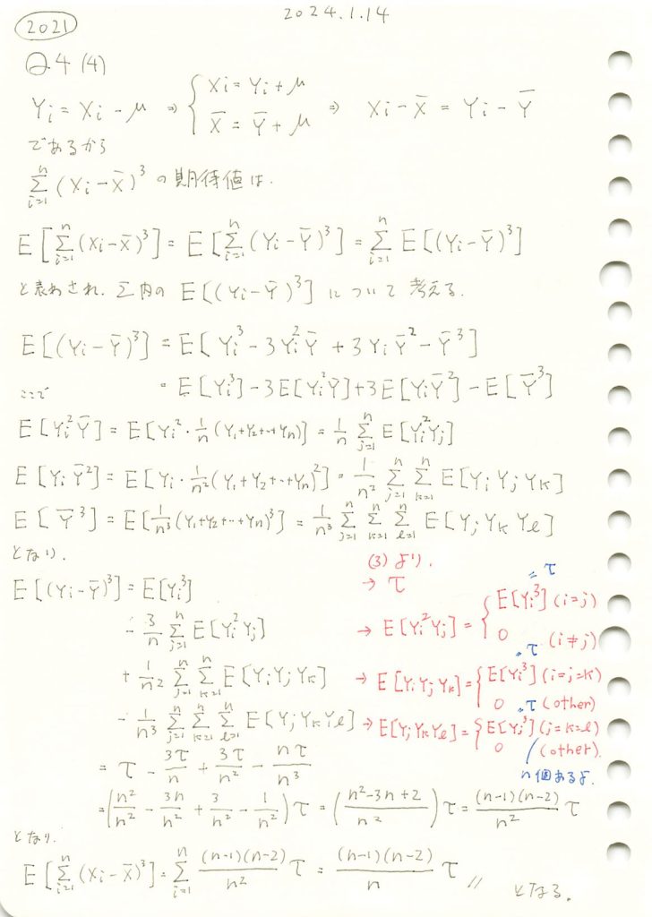
2021 Q4(4)
標本平均との差の3乗の和の期待値を求める問題をやりました。
コード
シミュレーションをして理論値と比較します
import numpy as np
import matplotlib.pyplot as plt

# パラメータの設定
n = 10  # サンプル数 (必要に応じて変更可能)
scale = 1.0  # 指数分布のスケールパラメータ(1/λ)
iterations = 10000  # シミュレーション回数

# シミュレーション結果を保存するリスト
sum_X_i_minus_X_bar_cubed_values = []

# シミュレーションを実行
for _ in range(iterations):
    # 指数分布に従う乱数を生成
    X = np.random.exponential(scale=scale, size=n)

    # 標本平均を計算
    X_bar = np.mean(X)

    # (X_i - X_bar)^3 の合計を計算
    sum_X_i_minus_X_bar_cubed = np.sum((X - X_bar)**3)
    sum_X_i_minus_X_bar_cubed_values.append(sum_X_i_minus_X_bar_cubed)

# 指数分布の三次中心モーメントを計算
tau = 2 * scale**3  # 指数分布における三次中心モーメント

# 理論値の計算
theoretical_value = (n - 1) * (n - 2) * tau / n

# シミュレーション結果の平均
simulated_mean = np.mean(sum_X_i_minus_X_bar_cubed_values)

# 結果を表示
print(f"理論値: {theoretical_value}")
print(f"シミュレーションによる平均: {simulated_mean}")

# 視覚化
plt.figure(figsize=(10, 6))
plt.hist(sum_X_i_minus_X_bar_cubed_values, bins=50, alpha=0.75, label='シミュレーション結果')
plt.axvline(simulated_mean, color='red', linestyle='dashed', linewidth=2, label=f'シミュレーション平均 = {simulated_mean:.2f}')
plt.axvline(theoretical_value, color='blue', linestyle='dashed', linewidth=2, label=f'理論値 = {theoretical_value:.2f}')
plt.xlabel('値')
plt.ylabel('頻度')
plt.title(r"$\sum_{i=1}^{n} (X_i - \overline{X})^3$ の分布 (指数分布)")
plt.legend()
plt.grid(True)
plt.show()
理論値: 14.4
シミュレーションによる平均: 14.499748799877718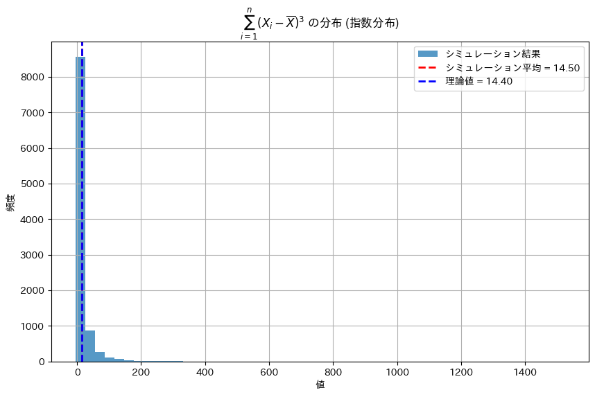
シミュレーションは理論値に近い値を示しました
コード中の三次中心モーメントの導出を下記に示します
指数分布の三次中心モーメント (=τ) の導出


![\mathbb{E}[X] = M_X'(0) = \frac{1}{\lambda}\\](https://statistics.blue/wp-content/ql-cache/quicklatex.com-0eeb17587006d727717a2d07b19a31c8_l3.png "Rendered by QuickLaTeX.com")
![\mathbb{E}[X^2] = M_X''(0) = \frac{2}{\lambda^2}\\](https://statistics.blue/wp-content/ql-cache/quicklatex.com-b714f63de924396702a8019d9177ab93_l3.png "Rendered by QuickLaTeX.com")
![\mathbb{E}[X^3] = M_X'''(0) = \frac{6}{\lambda^3}\\](https://statistics.blue/wp-content/ql-cache/quicklatex.com-1381a003c6f6bf2917cca8b0aeae08b6_l3.png "Rendered by QuickLaTeX.com")
![\mu_3 = \mathbb{E}[(X - \mathbb{E}[X])^3]\\](https://statistics.blue/wp-content/ql-cache/quicklatex.com-007569c2ddca853c072bcebbc93d3b5f_l3.png "Rendered by QuickLaTeX.com")
![\mu_3 = \mathbb{E}[X^3 - 3X^2\mathbb{E}[X] + 3X\mathbb{E}[X]^2 - \mathbb{E}[X]^3]\\](https://statistics.blue/wp-content/ql-cache/quicklatex.com-e91f4c20e51449fa69f145e549d0e5ce_l3.png "Rendered by QuickLaTeX.com")
![\mu_3 = \mathbb{E}[X^3] - 3\mathbb{E}[X^2]\mathbb{E}[X] + 3\mathbb{E}[X]\mathbb{E}[X]^2 - \mathbb{E}[X]^3\\](https://statistics.blue/wp-content/ql-cache/quicklatex.com-01157e322791acaff1d17f54d42b7f73_l3.png "Rendered by QuickLaTeX.com")
![\mu_3 = \mathbb{E}[X^3] - 3\mathbb{E}[X]\mathbb{E}[X^2] + 2\mathbb{E}[X]^3](https://statistics.blue/wp-content/ql-cache/quicklatex.com-62c10fe27755404dcd73de047024189e_l3.png "Rendered by QuickLaTeX.com")


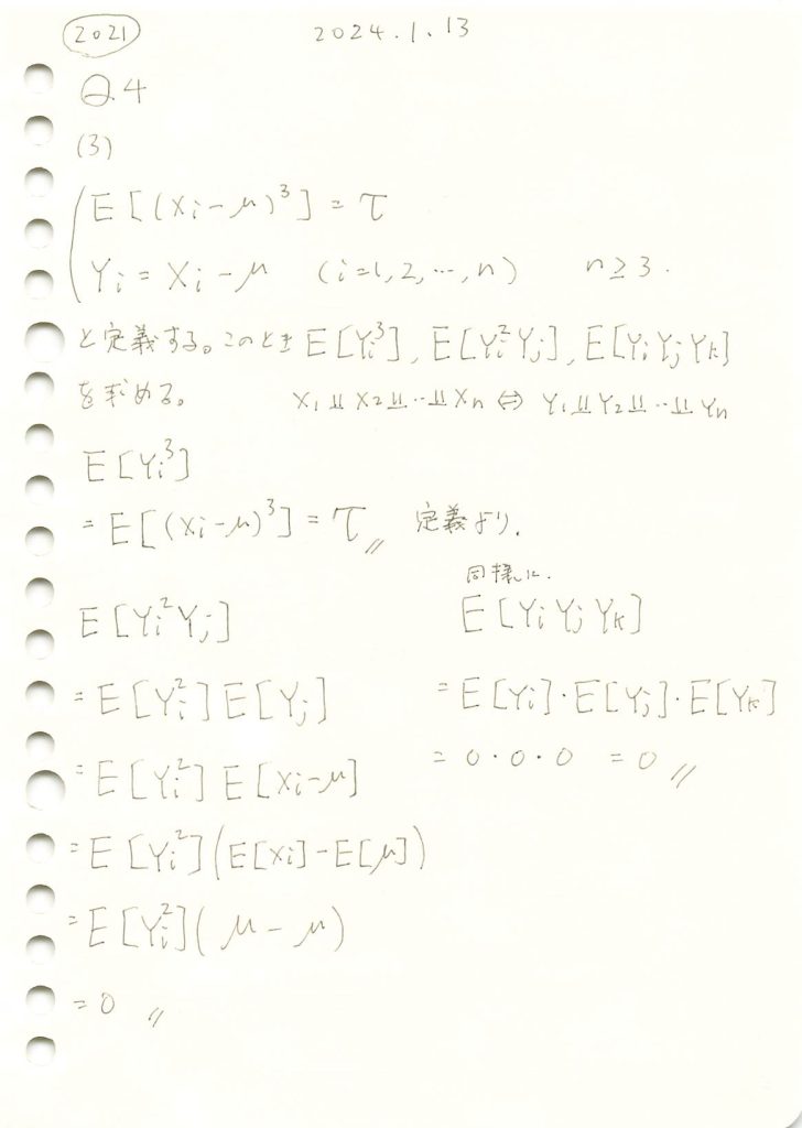
2021 Q4(3)
確率変数と母平均の差に関する期待値の計算をしました。
コード
Xiが正規分布(μ=0, σ=1)に従う場合
import numpy as np
import matplotlib.pyplot as plt

# パラメータの設定
n = 1000  # サンプル数
mu, sigma = 0, 1  # 正規分布の平均と標準偏差
iterations = 10000  # シミュレーション回数

# シミュレーション結果を保存するリスト
Y_i_cubed_values = []
Y_i_squared_Y_j_values = []
Y_i_Y_j_Y_k_values = []

# シミュレーションを実行
for _ in range(iterations):
    X_i = np.random.normal(mu, sigma, size=n)
    X_j = np.random.normal(mu, sigma, size=n)
    X_k = np.random.normal(mu, sigma, size=n)

    Y_i = X_i - mu
    Y_j = X_j - mu
    Y_k = X_k - mu

    Y_i_cubed_values.append(np.mean(Y_i**3))
    Y_i_squared_Y_j_values.append(np.mean(Y_i**2 * Y_j))
    Y_i_Y_j_Y_k_values.append(np.mean(Y_i * Y_j * Y_k))

# グラフを横に並べて表示
fig, axes = plt.subplots(1, 3, figsize=(18, 6))

# (1) E[Y_i^3] の分布
axes[0].hist(Y_i_cubed_values, bins=50, alpha=0.75)
axes[0].axvline(np.mean(Y_i_cubed_values), color='red', linestyle='dashed', linewidth=2, label='平均')
axes[0].set_title(r"正規分布における $E[Y_i^3]$ の分布")
axes[0].set_xlabel('値')
axes[0].set_ylabel('頻度')
axes[0].legend()

# (2) E[Y_i^2 Y_j] の分布
axes[1].hist(Y_i_squared_Y_j_values, bins=50, alpha=0.75)
axes[1].axvline(np.mean(Y_i_squared_Y_j_values), color='red', linestyle='dashed', linewidth=2, label='平均')
axes[1].set_title(r"正規分布における $E[Y_i^2 Y_j]$ の分布")
axes[1].set_xlabel('値')
axes[1].set_ylabel('頻度')
axes[1].legend()

# (3) E[Y_i Y_j Y_k] の分布
axes[2].hist(Y_i_Y_j_Y_k_values, bins=50, alpha=0.75)
axes[2].axvline(np.mean(Y_i_Y_j_Y_k_values), color='red', linestyle='dashed', linewidth=2, label='平均')
axes[2].set_title(r"正規分布における $E[Y_i Y_j Y_k]$ の分布")
axes[2].set_xlabel('値')
axes[2].set_ylabel('頻度')
axes[2].legend()

# グラフを表示
plt.tight_layout()
plt.show()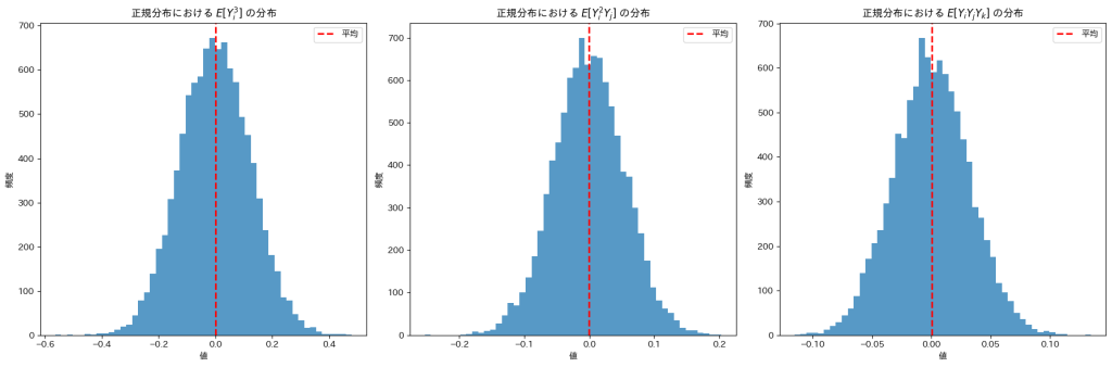
![E[Y_i^3],E[Y_i^2 Y_j],E[Y_i Y_j Y_k]](https://statistics.blue/wp-content/ql-cache/quicklatex.com-85bedb2efe9aa8ae96f7d7ef47a14a21_l3.png "Rendered by QuickLaTeX.com") は0になります
は0になります
Xiが指数分布(λ=1)に従う場合
import numpy as np
import matplotlib.pyplot as plt

# パラメータの設定
n = 1000  # サンプル数
scale = 1.0  # 指数分布のスケールパラメータ(1/λ)
iterations = 10000  # シミュレーション回数

# シミュレーション結果を保存するリスト
Y_i_cubed_values = []
Y_i_squared_Y_j_values = []
Y_i_Y_j_Y_k_values = []

# シミュレーションを実行
for _ in range(iterations):
    X_i = np.random.exponential(scale=scale, size=n)
    X_j = np.random.exponential(scale=scale, size=n)
    X_k = np.random.exponential(scale=scale, size=n)

    Y_i = X_i - np.mean(X_i)
    Y_j = X_j - np.mean(X_j)
    Y_k = X_k - np.mean(X_k)

    Y_i_cubed_values.append(np.mean(Y_i**3))
    Y_i_squared_Y_j_values.append(np.mean(Y_i**2 * Y_j))
    Y_i_Y_j_Y_k_values.append(np.mean(Y_i * Y_j * Y_k))

# グラフを横に並べて表示
fig, axes = plt.subplots(1, 3, figsize=(18, 6))

# (1) E[Y_i^3] の分布
axes[0].hist(Y_i_cubed_values, bins=50, alpha=0.75)
axes[0].axvline(np.mean(Y_i_cubed_values), color='red', linestyle='dashed', linewidth=2, label='平均')
axes[0].set_title(r"指数分布における $E[Y_i^3]$ の分布")
axes[0].set_xlabel('値')
axes[0].set_ylabel('頻度')
axes[0].legend()

# (2) E[Y_i^2 Y_j] の分布
axes[1].hist(Y_i_squared_Y_j_values, bins=50, alpha=0.75)
axes[1].axvline(np.mean(Y_i_squared_Y_j_values), color='red', linestyle='dashed', linewidth=2, label='平均')
axes[1].set_title(r"指数分布における $E[Y_i^2 Y_j]$ の分布")
axes[1].set_xlabel('値')
axes[1].set_ylabel('頻度')
axes[1].legend()

# (3) E[Y_i Y_j Y_k] の分布
axes[2].hist(Y_i_Y_j_Y_k_values, bins=50, alpha=0.75)
axes[2].axvline(np.mean(Y_i_Y_j_Y_k_values), color='red', linestyle='dashed', linewidth=2, label='平均')
axes[2].set_title(r"指数分布における $E[Y_i Y_j Y_k]$ の分布")
axes[2].set_xlabel('値')
axes[2].set_ylabel('頻度')
axes[2].legend()

# グラフを表示
plt.tight_layout()
plt.show()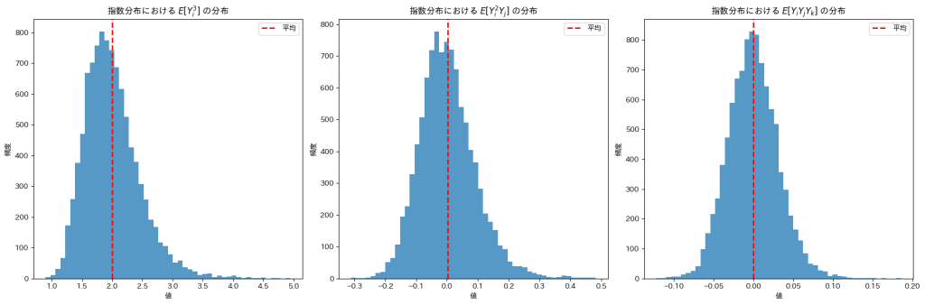
![E[Y_i^2 Y_j],E[Y_i Y_j Y_k]](https://statistics.blue/wp-content/ql-cache/quicklatex.com-bf7e90f87bbed6b8bc7009c4fea4e61c_l3.png "Rendered by QuickLaTeX.com") は0になりますが、
は0になりますが、![E[Y_i^3]](https://statistics.blue/wp-content/ql-cache/quicklatex.com-c3202786e2c4756a55bdf3837c41ffde_l3.png "Rendered by QuickLaTeX.com") は2付近の値をとっているようです。
は2付近の値をとっているようです。
Xiがガンマ分布(形状パラメータ=2, スケールパラメータ=2)に従う場合
import numpy as np
import matplotlib.pyplot as plt

# パラメータの設定
n = 1000  # サンプル数
shape, scale = 2.0, 2.0  # ガンマ分布の形状パラメータとスケールパラメータ
iterations = 10000  # シミュレーション回数

# シミュレーション結果を保存するリスト
Y_i_cubed_values = []
Y_i_squared_Y_j_values = []
Y_i_Y_j_Y_k_values = []

# シミュレーションを実行
for _ in range(iterations):
    X_i = np.random.gamma(shape, scale, size=n)
    X_j = np.random.gamma(shape, scale, size=n)
    X_k = np.random.gamma(shape, scale, size=n)

    Y_i = X_i - np.mean(X_i)
    Y_j = X_j - np.mean(X_j)
    Y_k = X_k - np.mean(X_k)

    Y_i_cubed_values.append(np.mean(Y_i**3))
    Y_i_squared_Y_j_values.append(np.mean(Y_i**2 * Y_j))
    Y_i_Y_j_Y_k_values.append(np.mean(Y_i * Y_j * Y_k))

# グラフを横に並べて表示
fig, axes = plt.subplots(1, 3, figsize=(18, 6))

# (1) E[Y_i^3] の分布
axes[0].hist(Y_i_cubed_values, bins=50, alpha=0.75)
axes[0].axvline(np.mean(Y_i_cubed_values), color='red', linestyle='dashed', linewidth=2, label='平均')
axes[0].set_title(r"ガンマ分布における $E[Y_i^3]$ の分布")
axes[0].set_xlabel('値')
axes[0].set_ylabel('頻度')
axes[0].legend()

# (2) E[Y_i^2 Y_j] の分布
axes[1].hist(Y_i_squared_Y_j_values, bins=50, alpha=0.75)
axes[1].axvline(np.mean(Y_i_squared_Y_j_values), color='red', linestyle='dashed', linewidth=2, label='平均')
axes[1].set_title(r"ガンマ分布における $E[Y_i^2 Y_j]$ の分布")
axes[1].set_xlabel('値')
axes[1].set_ylabel('頻度')
axes[1].legend()

# (3) E[Y_i Y_j Y_k] の分布
axes[2].hist(Y_i_Y_j_Y_k_values, bins=50, alpha=0.75)
axes[2].axvline(np.mean(Y_i_Y_j_Y_k_values), color='red', linestyle='dashed', linewidth=2, label='平均')
axes[2].set_title(r"ガンマ分布における $E[Y_i Y_j Y_k]$ の分布")
axes[2].set_xlabel('値')
axes[2].set_ylabel('頻度')
axes[2].legend()

# グラフを表示
plt.tight_layout()
plt.show()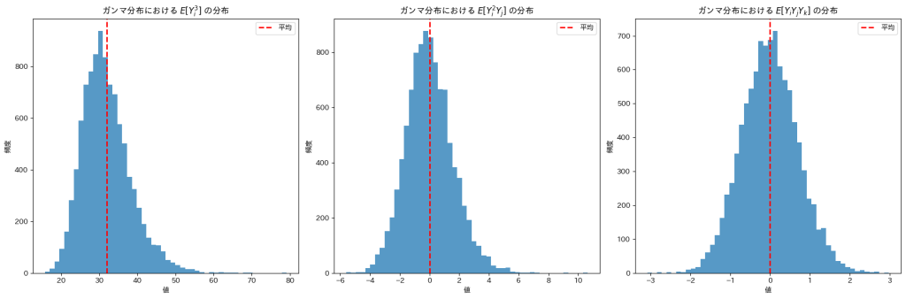
は0になりますが、は32付近の値をとっているようです。
2021 Q4(1)(2)
平均の分散と、同じ分布に従う2変数の差の3乗の期待値を求めました。
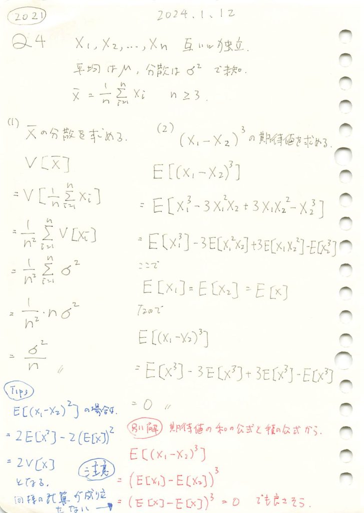
(1)標本平均の分散
# 2021 Q4(1)  2024.8.31

import numpy as np

# パラメータの設定
n = 100  # サンプル数
mu = 0  # 平均
sigma = 1  # 標準偏差
iterations = 10000  # シミュレーション回数

# 各シミュレーションで得た標本平均を格納するリスト
sample_means = []

for _ in range(iterations):
    # 正規分布に従う乱数を生成
    X = np.random.normal(loc=mu, scale=sigma, size=n)

    # 標本平均を計算
    X_bar = np.mean(X)
    sample_means.append(X_bar)

# 標本平均の分散を計算
estimated_variance_of_sample_mean = np.var(sample_means)

# 理論的な分散
theoretical_variance = sigma**2 / n

print(f"理論的な分散: {theoretical_variance}")
print(f"推定された標本平均の分散: {estimated_variance_of_sample_mean}")
理論的な分散: 0.01
推定された標本平均の分散: 0.009838287336429174
分布を見てみます
import numpy as np
import matplotlib.pyplot as plt

# パラメータの設定
n = 100  # サンプル数
mu = 0  # 平均
sigma = 1  # 標準偏差
iterations = 10000  # シミュレーション回数

# 分散の推定値を格納するリスト
estimated_variances = []

for _ in range(iterations):
    # 正規分布に従う乱数を生成
    X = np.random.normal(loc=mu, scale=sigma, size=n)

    # 標本平均の分散を計算
    estimated_variance = np.var(X) / n
    estimated_variances.append(estimated_variance)

# 理論的な分散
theoretical_variance = sigma**2 / n

# 視覚化
plt.figure(figsize=(10, 6))
plt.hist(estimated_variances, bins=100, alpha=0.75, label='推定された分散', range=(0.005, 0.015))
plt.axvline(theoretical_variance, color='red', linestyle='dashed', linewidth=2, label=f'理論的な分散 = {theoretical_variance}')
plt.xlabel('分散')
plt.ylabel('頻度')
plt.title(f'{iterations}回のシミュレーションにおける推定された分散の分布\n(サンプルサイズ = {n})')
plt.legend()
plt.grid(True)
plt.show()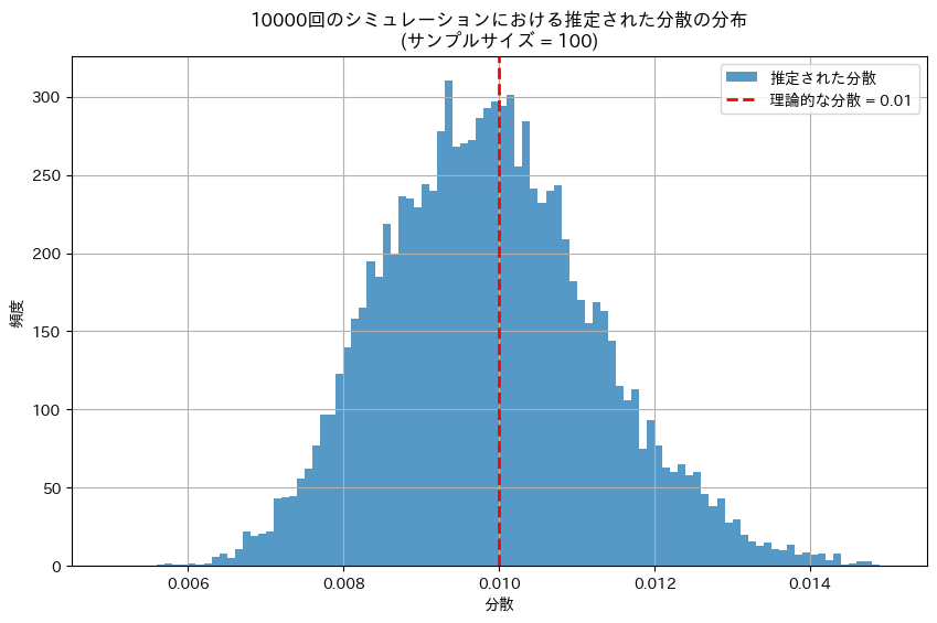
(2) 2変数の差の3乗の期待値
# 2021 Q4(1)  2024.8.31

import numpy as np

# パラメータの設定
n_simulations = 10000  # シミュレーション回数
mu = 0  # 平均
sigma = 1  # 標準偏差

# X1, X2を正規分布から生成
X1 = np.random.normal(loc=mu, scale=sigma, size=n_simulations)
X2 = np.random.normal(loc=mu, scale=sigma, size=n_simulations)

# (X1 - X2)^3を計算
expression = (X1 - X2)**3

# 期待値を計算
expected_value = np.mean(expression)

print(f"(X1 - X2)^3 の期待値: {expected_value}")
(X1 - X2)^3 の期待値: 0.044962030052379295分布を見てみます
import numpy as np
import matplotlib.pyplot as plt

# パラメータの設定
n = 10000  # シミュレーション回数
mu = 0  # 平均
sigma = 1  # 標準偏差

# (X1 - X2)^3 の推定値を格納するリスト
expected_values = []

for _ in range(n):
    # 正規分布に従う X1, X2 を生成
    X1 = np.random.normal(loc=mu, scale=sigma)
    X2 = np.random.normal(loc=mu, scale=sigma)

    # (X1 - X2)^3 を計算
    value = (X1 - X2)**3
    expected_values.append(value)

# 理論的な期待値
theoretical_expectation = 0

# 視覚化
plt.figure(figsize=(10, 6))
plt.hist(expected_values, bins=100, alpha=0.75, label='(X1 - X2)^3 の推定値', range=(-30, 30))
plt.axvline(theoretical_expectation, color='red', linestyle='dashed', linewidth=2, label=f'理論的な期待値 = {theoretical_expectation}')
plt.xlabel('値')
plt.ylabel('頻度')
plt.title(f'{n}回のシミュレーションにおける (X1 - X2)^3 の期待値の分布')
plt.legend()
plt.grid(True)
plt.show()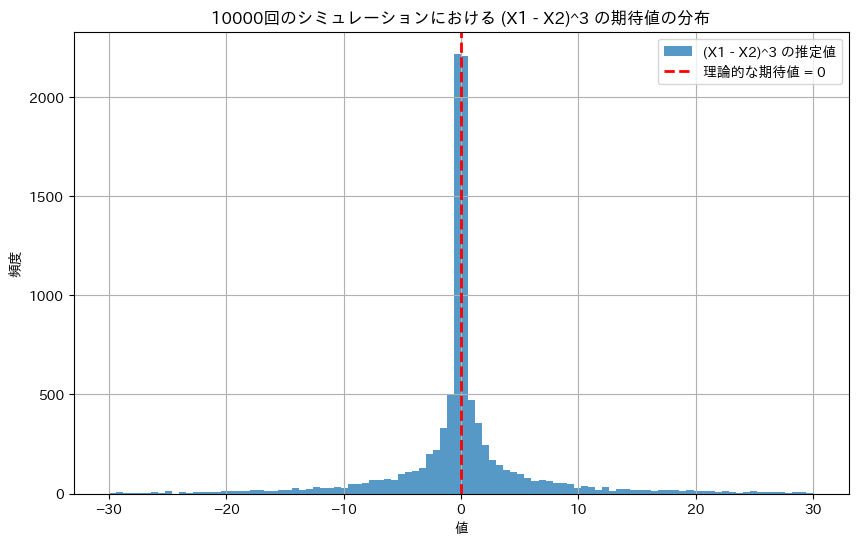
|X1-X2|が1より小さい場合は0付近に集中し、|X1-X2|が1より大きい場合は、三乗によって値が急激に増減する。分布は中心が尖って、左右対称になる。外れ値の影響を受けやすい。